neuroscicomplab: Bayesianische Statistik

Andrew Ellis

library(tidyverse)
library(rmarkdown)
library(kableExtra)

Einführung

Bisher haben wir:

Parameter geschätzt
- Binomial (Bernoulli) Modell
- Lineare Modelle mit kategorialem Prädiktor
Posterior Verteilung(en) zusammengefasst
- Credible Intervals
- Highest Posterior Density Intervals

Wir würden gerne Aussagen über die Wahrscheinlichkeiten von Modellen machen:

z.B. Modell 1 (M1) erklärt die Daten besser als Modell 2 (M2).
M1 ist wahrscheinlicher als M2

Solche Aussagen sind Modellvergleiche.

Welche Methoden kennen Sie, um Modelle zu vergleichen?

Diskutieren Sie anhand dieses Beispiels, wie Sie die Hypothese testen können, dass die Intervention einen Effekt hat.

library(tidyverse)
intervention <- rep(c('treat', 'control'), each = 5)
pre <- c(20, 10, 60, 20, 10, 50, 10, 40, 20, 10)
post <- c(70, 50, 90, 60, 50, 20, 10, 30, 50, 10)

dwide <- tibble(id = factor(1:10), 
            intervention, pre, post) %>% 
  mutate(diff = post - pre,
         id = as_factor(id), 
         intervention =  factor(intervention, levels = c("control", "treat")))
d <- dwide %>% 
  select(-diff) %>% 
  pivot_longer(cols = pre:post, names_to = "time", values_to = "score") %>% 
  mutate(time = as_factor(time))

Wir haben hier einen within (messwiederholten) Faktor (time), und einen between Faktor (intervention).

d %>% 
  ggplot(aes(time, score, color = intervention)) +
  geom_line(aes(group = id), linetype = 1, size = 1) +
  geom_point(size = 4) +
  scale_color_viridis_d(end = 0.8)

Mögliche Methoden

Hypothesentest, z.B.

t.test(diff ~ intervention,
       data = dwide)

m1 <- lmer(score ~ intervention + time + (1|id), 
                  data = d)
m2 <- lmer(score ~ intervention * time + (1|id), 
                  data = d)

Modellvergleiche
- Varianzaufklärung
- Informationskriterien
- Kreuzvalidierung

Wir lernen nun Methoden kennen, um mit Bayesianischen Modellen Modellvergleiche durchzuführen.

Bayesianische Modellvergleiche

Wir unterscheiden 3 verschiedene Methoden

Bayes Factors
Out of sample predictive accuracy:

Approximate leave-one-out cross validation (LOO)

Informationskriterien: widely application information criterion (WAIC)

Posterior predictive checking: > Konstruktion einer Teststatistik und Vergleich der aktuellen Daten mit generierten Daten aus der Posterior Predictive Distribution.

Heute schauen wir uns die erste Methode (Bayes Factors) an. Diese sind unter Statistikern sehr umstritten. Psychologen wollen Hypothesen testen (Evidenz für/gegen Hypothesen), während in anderen Bereichen dies weniger verbreitet ist.

Bayes factor

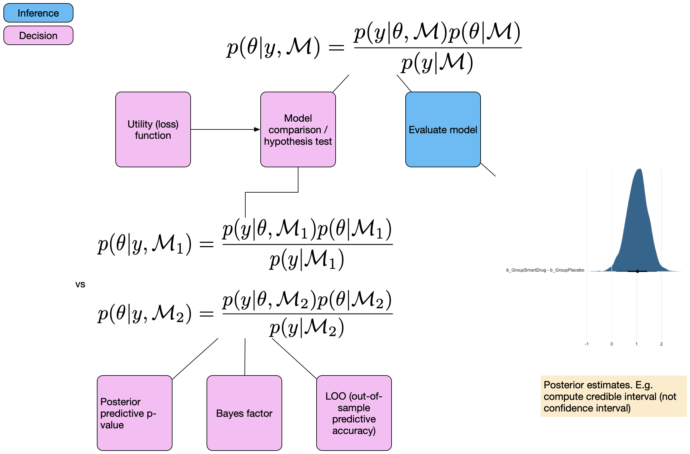
Bayes’ Theorem, mit expliziter Abhängigkeit der Parameter \(\mathbf{\theta}\) vom Modells \(\mathcal{M}\):

\[ p(\theta | y, \mathcal{M}) = \frac{p(y|\theta, \mathcal{M}) p(\theta | \mathcal{M})}{p(y | \mathcal{M})}\]

\(\mathcal{M}\) bezieht sich auf ein bestimmtes Modell.

\(p(y | \mathcal{M})\) ist die Wahrscheinlichkeit der Daten (marginal likelihood), über alle möglichen Parameterwerte des Modells \(\mathcal{M}\) integriert. Wir haben sie anfangs als Normierungskonstante bezeichnet.

\[ P(\theta|Data) = \frac{ P(Data|\theta) * P(\theta) } {P(Data)} \]

\[ P(\theta|Data) \propto P(Data|\theta) * P(\theta) \]

\[ p(y | \mathcal{M}) = \int_{\theta}{p(y | \theta, \mathcal{M}) p(\theta|\mathcal{M})d\theta} \] Bei der Berechnung der Marginal Likelihood muss über alle unter dem Modell möglichen Werte von \(\theta\) gemittelt werden.

Komplexität

Marginal Likelihood wird auch Model Evidence genannt. Sie hängt davon ab, welche Vorhersagen ein Model machen kann (warum?).
Ein Modell, welches viele Vorhersagen machen kann, ist ein komplexes Modell. Die meisten Vorhersagen werden aber falsch sein (warum?).

Komplexität hängt unter anderem ab von:

Anzahl Parameter im Modell
Prior Verteilungen der Parameter

Bei frequentistischen Modellen spielt nur die Anzahl Parameter eine Rolle.

Prior Verteilungen

Uninformative Priors machen viele Vorhersagen, vor allem in Gegenden des Parameterraums, in denen die Lieklihood niedrig ist.

prior <- dbeta(x = p_grid, shape1 = 1, shape2 = 1)
compute_posterior(likelihood, prior)

prior <- dbeta(x = p_grid, shape1 = 20, shape2 = 20)
compute_posterior(likelihood, prior)

prior <- dbeta(x = p_grid, shape1 = 2, shape2 = 40)
compute_posterior(likelihood, prior)

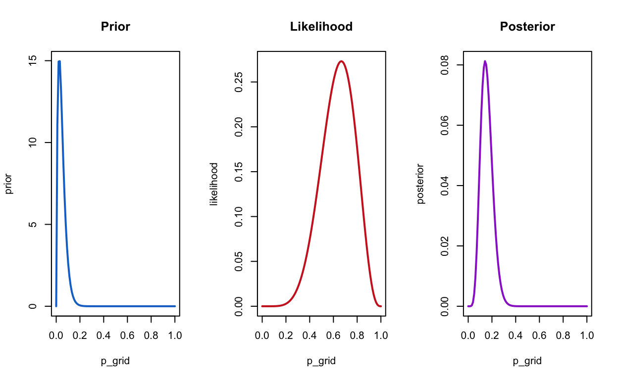
prior <- dbeta(x = p_grid, shape1 = 48, shape2 = 30)
compute_posterior(likelihood, prior)

Ockham’s Razor

Komplexe Modelle haben eine niedrigere Marginal Likelihood.
Wenn wir bei einem Vergleich mehrerer Modelle diejenigen Modelle mit höherer Marginal Likelihood bevorzugen, wenden wir das Prinzip der Sparsamkeit an.

Wir schreiben Bayes Theorem mit expliziten Modellen M1 und M2

\[ p(\mathcal{M}_1 | y) = \frac{P(y | \mathcal{M}_1) p(\mathcal{M}_1)}{p(y)} \]

und

\[ p(\mathcal{M}_2 | y) = \frac{P(y | \mathcal{M}_2) p(\mathcal{M}_2)}{p(y)} \]

Für Model \(\mathcal{M_m}\) ist die Posterior Wahrscheinlichkeit des Modells proportional zum Produkt der Marginal Likelihood und der A Priori Wahrscheinlichkeit.

Modellvergleich

Verhältnis der Modellwahrscheinlichkeiten:

\[ \frac{p(\mathcal{M}_1 | y) = \frac{P(y | \mathcal{M}_1) p(\mathcal{M}_1)}{p(y)}} {p(\mathcal{M}_2 | y) = \frac{P(y | \mathcal{M}_2) p(\mathcal{M}_2)}{p(y)}} \]

\(p(y)\) kann rausgekürzt werden.

\[\underbrace{\frac{p(\mathcal{M}_1 | y)} {p(\mathcal{M}_2 | y)}}_\text{Posterior odds} = \frac{P(y | \mathcal{M}_1)}{P(y | \mathcal{M}_2)} \cdot \underbrace{ \frac{p(\mathcal{M}_1)}{p(\mathcal{M}_2)}}_\text{Prior odds}\]

\(\frac{p(\mathcal{M}_1)}{p(\mathcal{M}_2)}\) sind die prior odds, und \(\frac{p(\mathcal{M}_1 | y)}{p(\mathcal{M}_2 | y)}\) sind die posterior odds.

Nehmen wir an, die Prior Odds seine \(1\), dann interessiert uns nur das Verhältnis der Marginal Likelihoods:

\[ \frac{P(y | \mathcal{M}_1)}{P(y | \mathcal{M}_2)} \]

Dieser Term ist der Bayes factor: der Term, mit dem die Prior Odds multipliziert werden. Er gibt an, unter welchem Modell die Daten wahrscheinlicher sind.

Wir schreiben \(BF_{12}\) - dies ist der Bayes factor für Modell 1 vs Modell 2.

\[ BF_{12} = \frac{P(y | \mathcal{M}_1)}{P(y | \mathcal{M}_2)}\]

\(BF_{12}\) gibt an, in welchem Ausmass die Daten \(\mathcal{M}_1\) bevorzugen, relativ zu \(\mathcal{M}_2\).

Beispiel: \(BF_{12} = 5\) heisst: die Daten sind unter Modell 1 5 Mal wahrscheinlicher als unter Modell 2

Klassifizierung

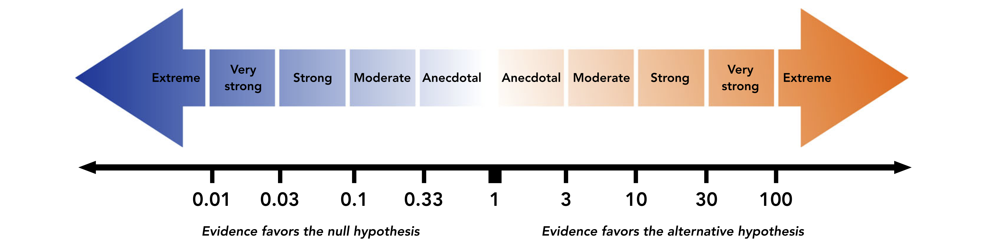
Bayes Factor

Sehr stark abhängig von den Prior Verteilungen der Parameter.
Ist nur für sehr simple Modelle einfach zu berechnen/schätzen.
Schätzmethoden
- Savage-Dickey Density Ratio mit Stan/brms
- Package BayesFactor (nur für allgemeine lineare Modelle)
- JASP: IM Prinzip ein GUI für BayesFactor
- Bridge sampling mit brms: schwieriger zu implementieren, aber für viele Modelle möglich.

Savage-Dickey Density Ratio

Wenn wir zwei genestete Modell vergleichen, wie z.B. ein Modell 1 mit einem frei geschätzten Parameter, und ein Nullmodell vergleichen, gibt es eine einfache Methode.

Unter dem Nullmodell (Nullhypothese): \(H_0: \theta = \theta_0\)

Unter Modell 1: \(H_0: \theta \neq \theta_0\)

Nun braucht der Parameter \(\theta\) unter Modell 1 eine Verteilung, z.B. \(\theta \sim \text{Beta}(1, 1)\)

Der Savage-Dickey Density Ratio Trick: wir betrachten nur Modell 1, und dividieren die Posterior Verteilung durch die Prior Verteilung an der Stelle \(\theta_0\).

Savage-Dickey Density Ratio

Wir schauen uns ein Beispiel aus Wagenmakers et al. (2010) an:

Sie beobachten, dass jemand 9 Fragen von 10 richtig beantwortet.

d <- tibble(s = 9, k = 10)

Unsere Frage: was ist die Wahrscheinlichkeit, dass das mit Glück ( \(\theta = 0.5\) ) passiert ist?

Table 1: Bayes Factors.
x	Prior	Posterior	BF01	BF10
0.5	1	0.107	0.107	9.309

Savage-Dickey Density Ratio

library(brms)

m1_formula <- bf(
  s | trials(k) ~ 0 + Intercept,
  family = binomial(link = "identity"))

get_prior(m1_formula, 
          data = d)

  prior class      coef group resp dpar nlpar bound       source
 (flat)     b                                            default
 (flat)     b Intercept                             (vectorized)

priors <- set_prior("beta(1, 1)", 
                   class = "b", 
                   lb = 0, ub = 1)

m1 <- brm(m1_formula,
         prior = priors,
         data = d,
         sample_prior = TRUE, #<<
         file = "models/05-m1")

summary(m1)

 Family: binomial 
  Links: mu = identity 
Formula: s | trials(k) ~ 0 + Intercept 
   Data: d (Number of observations: 1) 
Samples: 4 chains, each with iter = 2000; warmup = 1000; thin = 1;
         total post-warmup samples = 4000

Population-Level Effects: 
          Estimate Est.Error l-95% CI u-95% CI Rhat Bulk_ESS Tail_ESS
Intercept     0.83      0.10     0.58     0.97 1.00     1492     1345

Samples were drawn using sampling(NUTS). For each parameter, Bulk_ESS
and Tail_ESS are effective sample size measures, and Rhat is the potential
scale reduction factor on split chains (at convergence, Rhat = 1).

Posterior summary

m1 %>% 
  mcmc_plot(c("b_Intercept", "prior_b"))

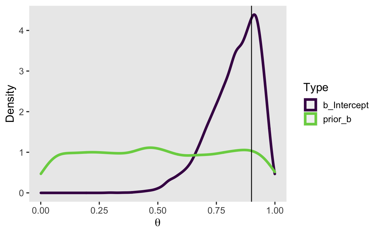
Prior und Posterior

.pull-left[

samples <- m1 %>% 
  posterior_samples("b")

Table 2: Six first rows of posterior samples.
b_Intercept	prior_b
0.94	0.19
0.93	0.87
0.92	0.59
0.91	0.06
0.71	0.04
0.68	0.86

samples %>% 
  pivot_longer(everything(), 
               names_to = "Type", 
               values_to = "value") %>%
  ggplot(aes(value, color = Type)) +
  geom_density(size = 1.5) +
  scale_color_viridis_d(end = 0.8) +
  labs(x = bquote(theta), y = "Density") +
  geom_vline(xintercept = .9)

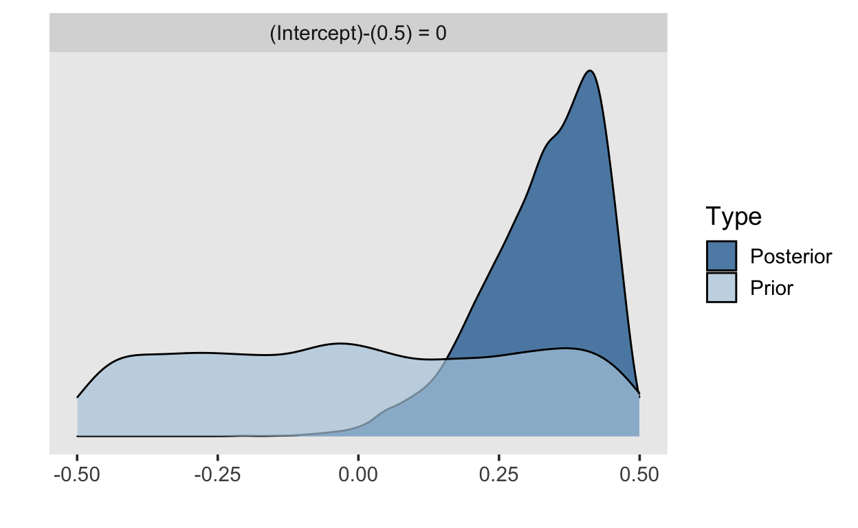
Savage-Dickey Density Ratio

Mit `brms`

h <- m1 %>% 
  hypothesis("Intercept = 0.5")

print(h, digits = 4)

Hypothesis Tests for class b:
             Hypothesis Estimate Est.Error CI.Lower CI.Upper Evid.Ratio Post.Prob Star
1 (Intercept)-(0.5) = 0   0.3275    0.1048   0.0767   0.4721     0.1028    0.0932    *
---
'CI': 90%-CI for one-sided and 95%-CI for two-sided hypotheses.
'*': For one-sided hypotheses, the posterior probability exceeds 95%;
for two-sided hypotheses, the value tested against lies outside the 95%-CI.
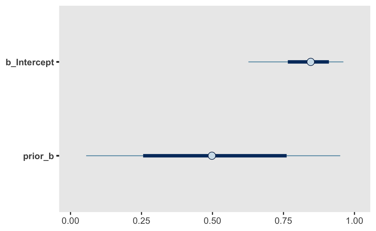
Posterior probabilities of point hypotheses assume equal prior probabilities.

Savage-Dickey Density Ratio

plot(h)

Bayes Factor für Vergleich von zwei Mittelwerten

smart = tibble(IQ = c(101,100,102,104,102,97,105,105,98,101,100,123,105,103,
                      100,95,102,106,109,102,82,102,100,102,102,101,102,102,
                      103,103,97,97,103,101,97,104,96,103,124,101,101,100,
                      101,101,104,100,101),
               Group = "SmartDrug")

placebo = tibble(IQ = c(99,101,100,101,102,100,97,101,104,101,102,102,100,105,
                        88,101,100,104,100,100,100,101,102,103,97,101,101,100,101,
                        99,101,100,100,101,100,99,101,100,102,99,100,99),
                 Group = "Placebo")

TwoGroupIQ <- bind_rows(smart, placebo)  %>%
    mutate(Group = fct_relevel(as.factor(Group), "Placebo"))

t.test(IQ ~ Group,
       data = TwoGroupIQ)


    Welch Two Sample t-test

data:  IQ by Group
t = -1.6222, df = 63.039, p-value = 0.1098
alternative hypothesis: true difference in means between group Placebo and group SmartDrug is not equal to 0
95 percent confidence interval:
 -3.4766863  0.3611848
sample estimates:
  mean in group Placebo mean in group SmartDrug 
               100.3571                101.9149

m2_formula <- bf(IQ ~ 1 + Group)

get_prior(m2_formula,
          data = TwoGroupIQ)

                  prior     class           coef group resp dpar
                 (flat)         b                               
                 (flat)         b GroupSmartDrug                
 student_t(3, 101, 2.5) Intercept                               
   student_t(3, 0, 2.5)     sigma                               
 nlpar bound       source
                  default
             (vectorized)
                  default
                  default

priors = c(set_prior("normal(0, 1)",
                    class = "b", coef = "GroupSmartDrug"))

m2 <- brm(m2_formula,
          prior = priors,
          data = TwoGroupIQ,
          cores = parallel::detectCores(),
          sample_prior = TRUE,
          file = here::here("models/05-m2-iq-bf"))

summary(m2)

 Family: gaussian 
  Links: mu = identity; sigma = identity 
Formula: IQ ~ 1 + Group 
   Data: TwoGroupIQ (Number of observations: 89) 
Samples: 4 chains, each with iter = 2000; warmup = 1000; thin = 1;
         total post-warmup samples = 4000

Population-Level Effects: 
               Estimate Est.Error l-95% CI u-95% CI Rhat Bulk_ESS
Intercept        100.76      0.61    99.58   101.96 1.00     4374
GroupSmartDrug     0.76      0.71    -0.64     2.17 1.00     4267
               Tail_ESS
Intercept          2977
GroupSmartDrug     3012

Family Specific Parameters: 
      Estimate Est.Error l-95% CI u-95% CI Rhat Bulk_ESS Tail_ESS
sigma     4.72      0.36     4.11     5.48 1.00     3654     2814

Samples were drawn using sampling(NUTS). For each parameter, Bulk_ESS
and Tail_ESS are effective sample size measures, and Rhat is the potential
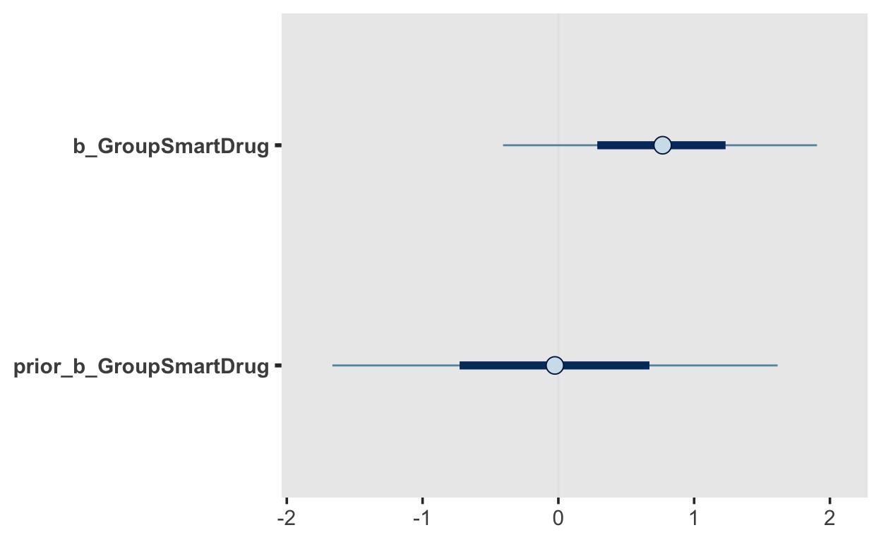
scale reduction factor on split chains (at convergence, Rhat = 1).

m2 %>% 
  mcmc_plot("GroupSmartDrug")

BF <- hypothesis(m2,
                hypothesis = 'GroupSmartDrug = 0')

BF

Hypothesis Tests for class b:
            Hypothesis Estimate Est.Error CI.Lower CI.Upper
1 (GroupSmartDrug) = 0     0.76      0.71    -0.64     2.17
  Evid.Ratio Post.Prob Star
1       0.81      0.45     
---
'CI': 90%-CI for one-sided and 95%-CI for two-sided hypotheses.
'*': For one-sided hypotheses, the posterior probability exceeds 95%;
for two-sided hypotheses, the value tested against lies outside the 95%-CI.
Posterior probabilities of point hypotheses assume equal prior probabilities.

1/BF$hypothesis$Evid.Ratio

[1] 1.23144

Speichern Sie den Dataframe mit der Funktion write_csv() TwoGroupIQ als CSV File.

write_csv(TwoGroupIQ, file = "SmartDrug.csv")

Laden Sie JASP herunter, und öffnen Sie das gespeicherte CSV File.

Führen Sie in JASP einen Bayesian t-Test durch.

Warum erhalten Sie nicht denselben Bayes Factor wie JASP?
Probieren Sie verschiedene Prior Verteilungen aus.
Versuchen Sie, das Ergebnis in Worten zusammenzufassen. Was sagt der Bayes Factor aus?

Wagenmakers, Eric-Jan, Tom Lodewyckx, Himanshu Kuriyal, and Raoul Grasman. 2010. “Bayesian Hypothesis Testing for Psychologists: A Tutorial on the Savage–Dickey Method.” Cognitive Psychology 60 (3): 158–89. https://doi.org/10.1016/j.cogpsych.2009.12.001.

Bayesianische Statistik

Einführung

Mögliche Methoden

Bayesianische Modellvergleiche

Bayes factor

Komplexität

Prior Verteilungen

Ockham’s Razor

Modellvergleich

Klassifizierung

Bayes Factor

Savage-Dickey Density Ratio

Savage-Dickey Density Ratio

Savage-Dickey Density Ratio

Posterior summary

Prior und Posterior

Savage-Dickey Density Ratio

Mit `brms`

Savage-Dickey Density Ratio

Bayes Factor für Vergleich von zwei Mittelwerten

References

Corrections

Reuse

Citation

Bayesianische Statistik

Einführung

Mögliche Methoden

Bayesianische Modellvergleiche

Bayes factor

Komplexität

Prior Verteilungen

Ockham’s Razor

Modellvergleich

Klassifizierung

Bayes Factor

Savage-Dickey Density Ratio

Savage-Dickey Density Ratio

Savage-Dickey Density Ratio

Posterior summary

Prior und Posterior

Savage-Dickey Density Ratio

Mit brms

Savage-Dickey Density Ratio

Bayes Factor für Vergleich von zwei Mittelwerten

References

Corrections

Reuse

Citation

Mit `brms`