Bayesianische Statistik

Von Grid Approximation zu Sampling

Zusammenfassung: Letzte Sitzung

• Parameterschätzung: Wahrscheinlichkeitsparameter einer Binomialverteilung
• Beta Verteilungen
• Grid Approximation

Bayes’ Theorem

\[ P(\theta|Data) = \frac{ P(Data|\theta) * P(\theta) } {P(Data)} \] oder ohne Normalisierungskonstante:

\[ P(\theta|Data) \propto P(Data|\theta) * P(\theta) \]

Parameterschätzung: Parameter einer Binomialverteilung

Die Binomial Likelihood ist gegeben durch

\[ P(x = k) = {n \choose k} \theta^k (1-\theta)^{n-k} \]

wins <- 6
games <- 9

Maximum Likelihood Schätzung

theta <- wins/games
theta

[1] 0.6666667

library(tidyverse)

tibble(x = seq(from = 0, to = 1, by = .01)) %>% 
  mutate(density = dbinom(6, 9, x)) %>% 
  
  ggplot(aes(x = x, ymin = 0, ymax = density)) +
  geom_ribbon(size = 0, alpha = 1/4, fill = "steelblue") +
  geom_vline(xintercept = theta, linetype = 2, size = 1.2) +
  scale_y_continuous(NULL, breaks = NULL) +
  coord_cartesian(xlim = c(0, 1)) +
  xlab("Wahrscheinlichkeit") +
  theme(panel.grid = element_blank(),
        legend.position = "none")

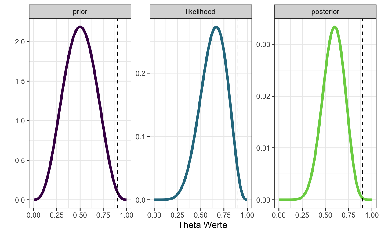
n_points <- 100
theta_grid <- seq(from = 0 , to = 1 , length.out = n_points)

likelihood <- dbinom(wins , size = games , prob = theta_grid)

prior <- dbeta(x = theta_grid, shape1 = 4,  shape2 = 4)

unstandardized_posterior <- likelihood * prior
posterior <- unstandardized_posterior / sum(unstandardized_posterior)

d <- tibble(theta_grid, prior, likelihood, posterior)

d %>%
  pivot_longer(-theta_grid, names_to = "distribution", values_to = "density") %>% 
  mutate(distribution = as_factor(distribution)) %>% 
  ggplot(aes(theta_grid, density, color = distribution)) +
  geom_line(size = 1.5) +
  geom_vline(xintercept = 9/10, linetype = "dashed") +
  scale_color_viridis_d(end = 0.8) +
  xlab("Theta Werte") +
  ylab("") +
  facet_wrap(~distribution, scales = "free_y") +
  theme_bw() +
  theme(legend.position = "none")

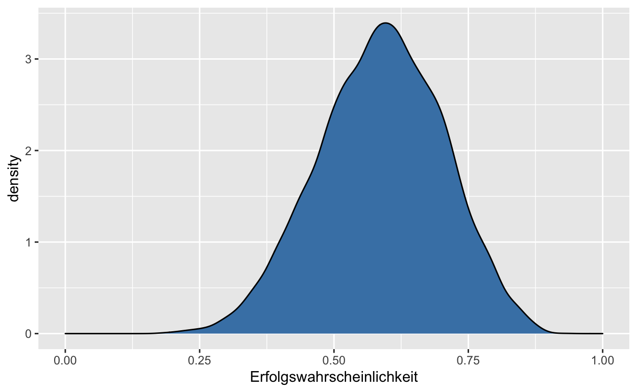
Posterior Verteilungen zusammenfassen

Samples aus dem Posterior ziehen:

n_samples <- 1e4
set.seed(3) # wegen Reproduzierbarkeit

library(rmarkdown)

d %>%
    paged_table(options = list(rows.print = 6))

samples <-
  d %>% 
  slice_sample(n = n_samples, weight_by = posterior, replace = TRUE) %>%
  mutate(sample_number = 1:n())

samples %>%
    paged_table(options = list(rows.print = 6))

samples %>%
  ggplot(aes(x = sample_number, y = theta_grid)) +
  geom_point(alpha = 1/10) +
  scale_y_continuous("Erfolgswahrscheinlichkeit", limits = c(0, 1)) +
  xlab("sample number")

Intervalle mit definierten Endpunkten

Posterior Approximation

sum(posterior[theta_grid > 0.5])

[1] 0.7728132

d %>% 
  filter(theta_grid > .5) %>% 
  summarise(sum = sum(posterior)) 

# A tibble: 1 x 1
    sum
  <dbl>
1 0.773

Intervalle mit definierten Endpunkten

Posterior Samples

samples %>% #<<
  filter(theta_grid > .5) %>% #<<
  summarise(sum = n() / n_samples) #<<

# A tibble: 1 x 1
    sum
  <dbl>
1 0.773

samples %>% 
  count(theta_grid > .5) %>% 
  mutate(probability = n / sum(n))

# A tibble: 2 x 3
  `theta_grid > 0.5`     n probability
  <lgl>              <int>       <dbl>
1 FALSE               2273       0.227
2 TRUE                7727       0.773

Intervalle mit definierter Masse

Quantile

quantile(samples$theta_grid, prob = c(.25, .75))

      25%       75% 
0.5050505 0.6666667 

library(tidybayes)
median_qi(samples$theta_grid, .width = .5)

          y      ymin      ymax .width .point .interval
1 0.5959596 0.5050505 0.6666667    0.5 median        qi

library(tidybayes)
median_qi(samples$theta_grid, .width = c(.5, .8, .99))

          y      ymin      ymax .width .point .interval
1 0.5959596 0.5050505 0.6666667   0.50 median        qi
2 0.5959596 0.4343434 0.7373737   0.80 median        qi
3 0.5959596 0.2929293 0.8484848   0.99 median        qi

Highest Posterior Density (HPDI)

mode_hdi(samples$theta_grid, .width = .5)

          y      ymin      ymax .width .point .interval
1 0.5961325 0.5151515 0.6666667    0.5   mode       hdi

hdi(samples$theta_grid, .width = .5)

          [,1]      [,2]
[1,] 0.5151515 0.6666667

library(patchwork)

p1 <-
  d %>% 
  ggplot(aes(x = theta_grid)) +
  # check out our sweet `qi()` indexing
  geom_ribbon(data = d %>% filter(theta_grid > qi(samples$theta_grid, .width = .5)[1] & 
                                    theta_grid < qi(samples$theta_grid, .width = .5)[2]),
              aes(ymin = 0, ymax = posterior),
              fill = "grey75") +
  geom_line(aes(y = posterior)) +
  labs(subtitle = "50% Percentile Interval",
       x = "Erfolgswahrscheinlichkeit",
       y = "density")


p2 <-
  d %>% 
  ggplot(aes(x = theta_grid)) +
  geom_ribbon(data = . %>% filter(theta_grid > hdi(samples$theta_grid, .width = .5)[1] & 
                                    theta_grid < hdi(samples$theta_grid, .width = .5)[2]),
              aes(ymin = 0, ymax = posterior),
              fill = "grey75") +
  geom_line(aes(y = posterior)) +
  labs(subtitle = "50% HPDI",
       x = "Erfolgswahrscheinlichkeit",
       y = "density")

p1 | p2

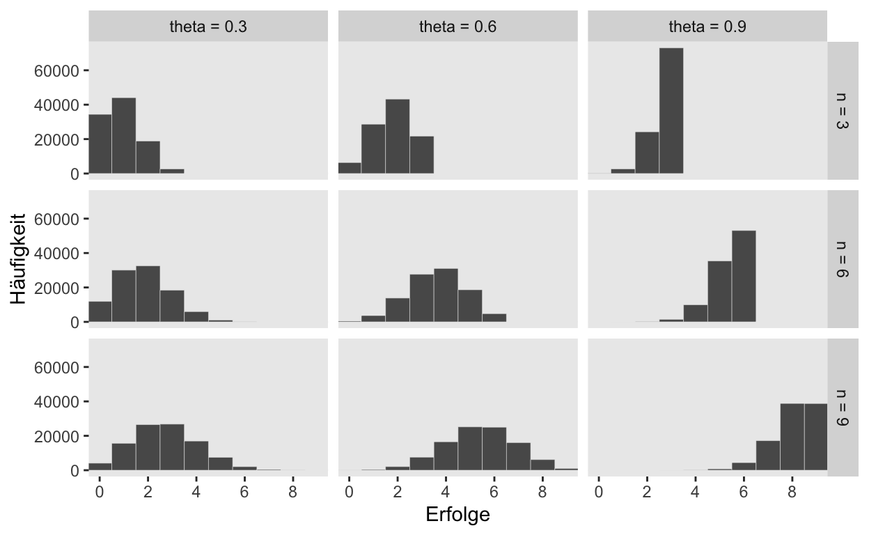
Sampling: Simulation

n_draws <- 1e5

simulate_binom <- function(n, probability) {
  set.seed(3)
  rbinom(n_draws, size = n, prob = probability) 
}

d <-
  crossing(n           = c(3, 6, 9),
           probability = c(.3, .6, .9)) %>% 
  mutate(draws = map2(n, probability, simulate_binom)) %>% 
  ungroup() %>% 
  mutate(n           = str_c("n = ", n),
         probability = str_c("theta = ", probability)) %>% 
  unnest(draws)

d %>% 
  ggplot(aes(x = draws)) +
  geom_histogram(binwidth = 1, center = 0,
                 color = "grey92", size = 1/10) +
  scale_x_continuous("Erfolge",
                     breaks = seq(from = 0, to = 9, by = 2)) +
  ylab("Häufigkeit") +
  coord_cartesian(xlim = c(0, 9)) +
  theme(panel.grid = element_blank()) +
  facet_grid(n ~ probability)

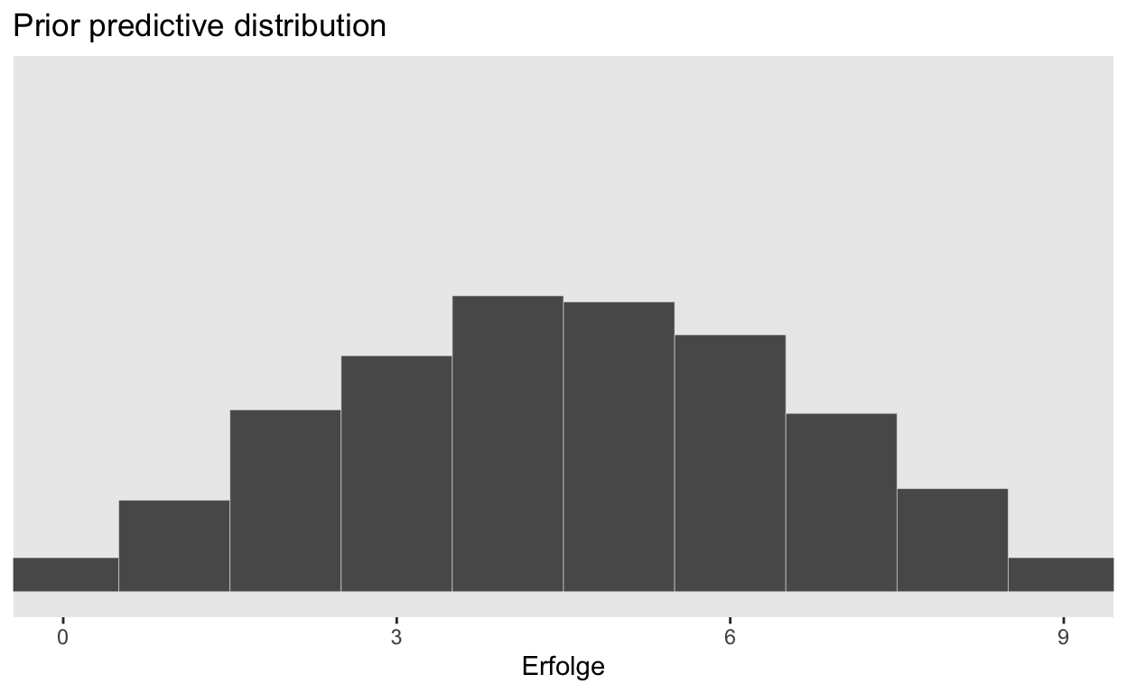
Prior Predictive Distribution

Posterior Predictive Distribution

Graphical model

Binomial Model

Grafische Darstellung des Generativen Modells:

Figure 1: Graphical Model für binomialverteilte Daten.

Figure 2: Graphical Model für bernoulliverteilte Daten.

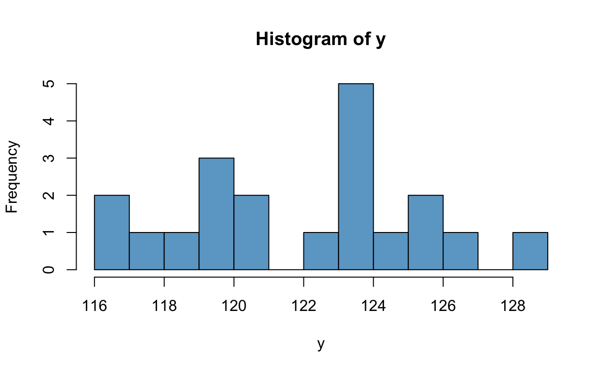
Gaussian model

Grafische Darstellung eines Generativen Modells mit normalverteilten Daten:

Figure 3: Graphical Model für normalverteilte Daten.

3

n <- 20

mu_sigma <- 5

set.seed(6)
mu <- rnorm(n = 1, mean = 120, 
            sd = mu_sigma)
sigma <- runif(n = 1, 1, 10)
y <- rnorm(n = n, mean = mu, 
           sd = sigma) %>% 
     round(2)

hist(y, col = 'skyblue3', breaks = 10) 

Posterior Inference

// The input data is a vector 'y' of length 'N'.
data {
  int<lower=0> N;
  vector[N] y;
}

// The parameters accepted by the model. Our model
// accepts two parameters 'mu' and 'sigma'.
parameters {
  real mu;
  real<lower=0> sigma;
}

// The model to be estimated. We model the output
// 'y' to be normally distributed with mean 'mu'
// and standard deviation 'sigma'.
model {
  mu ~ normal(120, 5);
  sigma ~ uniform(1, 10);
  y ~ normal(mu, sigma);
}

library(brms)
d <- tibble(y)

priors <- set_prior("normal(120, 5)", class = "Intercept") +
    set_prior("uniform(1, 10)", class = "sigma")

fit <- brm(y ~ 1,
           family = gaussian,
           prior = priors,
           data = d,
           cores = parallel::detectCores())

brms Model

library(brms)
d <- tibble(y)

get_prior(y ~ 1,
          family = gaussian,
          data = d)

                  prior     class coef group resp dpar nlpar bound
 student_t(3, 123, 4.4) Intercept                                 
   student_t(3, 0, 4.4)     sigma                                 
  source
 default
 default

priors <- set_prior("normal(120, 5)", class = "Intercept") +
  set_prior("cauchy(0, 1)", class = "sigma")

m <- brm(y ~ 1,
           family = gaussian,
           prior = priors,
           data = d,
           cores = parallel::detectCores(),
           file = "models/model_1")

summary(m)

Parameter werden durch Mittelwert, SD (Est.Error), 2-seitige 95% Credible intervals der Posterior-Verteilung zusammengefasst.

plot(m)

library(tidybayes)

m %>%
  spread_draws(b_Intercept) %>% 
  median_qi(.width = c(.50, .80, .95)) %>% 
  kableExtra::kbl()

b_Intercept	.lower	.upper	.width	.point	.interval
121.9501	121.4131	122.4658	0.50	median	qi
121.9501	120.9458	122.9398	0.80	median	qi
121.9501	120.4171	123.4596	0.95	median	qi

m %>%
  spread_draws(b_Intercept) %>%
  ggplot(aes(x = b_Intercept)) +
  stat_halfeye(.width = c(.50, .80, .95))