Bayesianische Statistik

Teil 3: Lineare Modelle mit brms

Parameterschätzung mit Linearen Modellen

Mittelwert und Standardabweichung einer Normalverteilung schätzen

Wir haben 3 Datenpunkte, von denen wir annehmen können, dass sie aus einer Normalverteilung kommen. Die drei Werte sind \(y_1 = 85\), \(y_2 = 100\), und \(y_3 = 115\). Die Wahrscheinlichkeit eines Datenpunktes is gegeben durch

\[ p(y | \mu, \sigma) = \frac{1}{Z} exp \left(- \frac{1}{2} \frac{(y-\mu)^2}{\sigma^2}\right) \]

\[ Z = \sigma \sqrt{2\pi} \] ist eine Normalisierungskonstante.

Damit können wir die Wahrscheinlichkeit eines Datenpunktes berechnen, wenn wir die Parameter \(\mu\) und \(\sigma\) kennen. Unter der Annahme, dass die drei Datenpunkte unabhängig sind, ist die Wahrscheinlichkeit der Daten das Produkt der Einzelwahrscheinlichkeiten.

Wie aber finden wir die beiden Parameter der Normalverteilung, \(\mu\) und \(\sigma\)?

Graphical model

Wir können wir schon im letzten Kapitel das Problem als Graphical Model darstellen. Dies hilft, das Problm zu veranschaulichen; vor allem wenn wir komplexere Probleme betrachten, kann dies hilfreich sein.

Figure 1: Graphical Model für normalverteilte Daten.

Die Variablen in diesem Modell sind:

\[ \mu \sim ??? \] \[ \sigma \sim ??? \] \[ y \sim N(\mu, \sigma) \]

\(y\) ist eine beobachtete Variable, und \(\mu\) und \(\sigma\) sind parameter, welche geschätzt werden müssen. Dies können wir mit der Maximum-Likelihood Methode machen, um Punktschätzungen zu erhalten. Der folgende Code illustriert, wie das ungefähr funktioniert. Wir suche eine Kombination von \(\mu\) und \(\sigma\), für welceh die Wahrscheinlichkeit am grössten ist, genau diese drei Dantepunkte zu beobachten. Anstatt alle möglichen Werte zu betrachten, wie in der Maximum-Likelihood Methode, nehmen wir drei Beispielswerte für \(\mu\), \(87.8, 100\) und \(112\), und drei Werte für \(\sigma\), \(7.35, 12.2\) und \(18.4\). Wir erstellen dann die 9 möglichen Kombinationen dieser Werte, und benutzten ein Grid (von 50 bis 150) für die möglichen Datenpunkte.

library(tidyverse)

sequence_length <- 100

d1 <- crossing(y = seq(from = 50, to = 150, length.out = sequence_length),
              mu = c(87.8, 100, 112),
              sigma = c(7.35, 12.2, 18.4)) %>%
    mutate(density = dnorm(y, mean = mu, sd = sigma),
           mu = factor(mu, labels = str_c("mu==", c(87.8, 100, 112))),
           sigma = factor(sigma, 
                          labels = str_c("sigma==", c(7.35, 12.2, 18.4))))

Dieser Code dient dazu, ein Theme für ggplot zu erstellen.

theme_set(
  theme_bw() +
    theme(text = element_text(color = "white"),
          axis.text = element_text(color = "black"),
          axis.ticks = element_line(color = "white"),
          legend.background = element_blank(),
          legend.box.background = element_rect(fill = "white",
                                               color = "transparent"),
          legend.key = element_rect(fill = "white",
                                    color = "transparent"),
          legend.text = element_text(color = "black"),
          legend.title = element_text(color = "black"),
          panel.background = element_rect(fill = "white",
                                          color = "white"),
          panel.grid = element_blank()))

In Grafik 2 werden nun die 9 Kombinationen, und die 3 beobachteten Datenpunkte (in Rot) dargestellt. Die Paratemeter \(\mu\) und \(\sigma\) definieren jeweils eine Normalverteilung, und die gestrichelte Linie zeigt die Wahrscheinlichkeit eines Datenpunktes unter dieser Verteilung. Die Wahrscheinlichkeit der Daten ist gegeben durch das Produkt der Wahrscheinlichkeiten. Diejenigen Paramterwerte, welche die Wahrscheinlichkeit maximieren, “gewinnen.” In diesem Beispiel wäre das die mittlere Verteilung.

d1 %>% 
  ggplot(aes(x = y)) +
  geom_ribbon(aes(ymin = 0, ymax = density),
              fill = "steelblue") +
  geom_vline(xintercept = c(85, 100, 115), 
             linetype = 3, color = "white") +
  geom_point(data = tibble(y = c(85, 100, 115)),
             aes(y = 0.002),
             size = 2, color = "red") +
  scale_y_continuous(expression(italic(p)(italic(y)*"|"*mu*", "*sigma)), 
                     expand = expansion(mult = c(0, 0.05)), breaks = NULL) +
  ggtitle("Welche Normalverteilung?") +
  coord_cartesian(xlim = c(60, 140)) +
  facet_grid(sigma ~ mu, labeller = label_parsed) +
  theme_bw() +
  theme(panel.grid = element_blank())

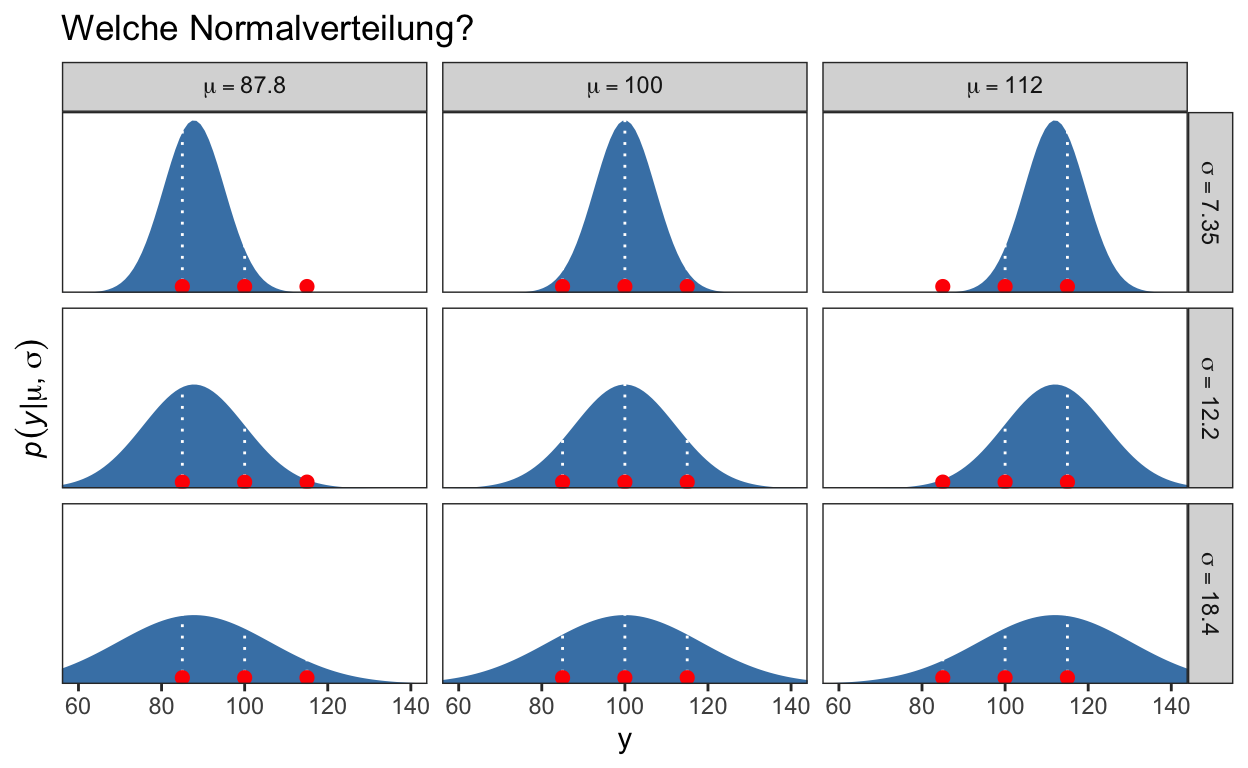
Figure 2: Kombinationen von \(\mu\) und \(\sigma\) Parameterwerten.

Beispiel: t-Test

Um die Parameter einer Normalverteilung mittels Markov Chain Monte Carlo Sampling Bayesian zu schätzen, nehmen wir ein Beispiel aus dem Buch Doing Bayesian Data Analysis (Kruschke 2015).

Wir haben IQ Scores einer Stichprobe, welche eine “Smart Drug” konsumiert hat. IQ Werte sind so normiert, dass wir in der Bevölkerung einen Mittelwert von 100, und eine SD von 15 haben. Nun wollen wir wissen, ob und wie sich die “Smart Drug” Gruppe von von diesem erwarteten Mittelwert unterscheidet. Gleichzeitig haben wir auch eine Gruppe, welche ein Placebo konsumiert hat.

Wir können die Daten von Hand eingeben, und zu einem Dataframe zusammenfügen.

smart = tibble(IQ = c(101,100,102,104,102,97,105,105,98,101,100,123,105,103,
                      100,95,102,106,109,102,82,102,100,102,102,101,102,102,
                      103,103,97,97,103,101,97,104,96,103,124,101,101,100,
                      101,101,104,100,101),
               Group = "SmartDrug")

placebo = tibble(IQ = c(99,101,100,101,102,100,97,101,104,101,102,102,100,105,
                        88,101,100,104,100,100,100,101,102,103,97,101,101,100,101,
                        99,101,100,100,101,100,99,101,100,102,99,100,99),
                 Group = "Placebo")

TwoGroupIQ <- bind_rows(smart, placebo) %>%
    mutate(Group = fct_relevel(as.factor(Group), "Placebo"))

Mit diesen Daten könnten wir einen t-Test machen, um die Mittelwerte der beiden Gruppen zu vergleichen. Die Mittelwertem sowie die beiden Standardabweichungen, können wir so schätzen.

Diese entsprechen den Maximum-Likelihood Schätzungen.

library(kableExtra)

TwoGroupIQ %>%
  group_by(Group) %>%
  summarise(mean = mean(IQ),
            sd = sd(IQ)) %>%
  mutate(across(where(is.numeric), round, 2)) %>% 
  kbl() %>%
  kable_styling(bootstrap_options = c("striped", "hover"))

Group	mean	sd
Placebo	100.36	2.52
SmartDrug	101.91	6.02

Die Smart Drug Gruppe hat einen leicht grösseren Mittelwert, aber auch eine grössere Standardabweichung, weshlab wir hier einen Welch-Test einem t-Test vorziehen würden.

t.test(IQ ~ Group,
       data = TwoGroupIQ)

    Welch Two Sample t-test

data:  IQ by Group
t = -1.6222, df = 63.039, p-value = 0.1098
alternative hypothesis: true difference in means between group Placebo and group SmartDrug is not equal to 0
95 percent confidence interval:
 -3.4766863  0.3611848
sample estimates:
  mean in group Placebo mean in group SmartDrug 
               100.3571                101.9149 

Dieser Welch-Test zeigt keine signifikante Mittelwertsdifferenz, mit einem p-Wert von \(0.1098\).

Mit diesem nicht-signifikanten Welch-Test gibt es nun nicht viele Möglichkeiten, weiterzufahren. Slebstverständlich hätten wir die Power dieses Test erhöhen können, aber nachdem die Daten gesammelt wurden, ist diese Erkenntnis nicht sehr hilfreich.

Smart Drug Gruppe

Wir ignorieren zunächst die Kontrollgruppe, und versuchen, die Parameter der Smart Drug Gruppe mit dem brms Package zu schätzen.

Wir erstelln zuerst einen Subdatensatz:

d <- TwoGroupIQ %>% 
  filter(Group == "SmartDrug") %>% 
  mutate(Group = fct_drop(Group))

d %>% 
  ggplot(aes(x = IQ)) +
  geom_histogram(fill = "skyblue3", binwidth = 1) +
  scale_y_continuous(expand = expansion(mult = c(0, 0.05))) + 
  theme_tidybayes()

Parameter schätzen mit brms

Wir wollen nun einen Mittelwert, und eine Standardabweichung mit brms schätzen. Bevor wir anfangen, überlegen wir uns zuerst, welche Prior Verteilungen denn überhaupt in Frage kommen. Für dieses Modell kennen wir bereits die Parameter, die wir schätzen müssen, aber in späteren Kapiteln werden wir es mir komplexeren Modellen zu tun haben, bei denen es nicht so offensichtilich ist.

Priors

Glücklicherweise bietet brms uns hier sehr viel Hilfe. Für die meisten Fälle können wir uns sogar darauf verlassen, dass die Default Priors genügen, so dass wir nicht einmal selber Priors definieren müssten. Es ist aber besser, wenn wir lernen, selber Prior Verteilungen zu definieren. In brms gibt es eine Funktion, get_prior(), mit welcher wir herausfinden können, welche Parameter Prior Verteilungen brauchen, und was die Defaults sind.

library(brms)

Diese Funktion nimmt als Argumente eine Formel, welche ein Regressionmodell spezifiert, und einen Dataframe. Alle weiteren Argumente sind optional. INdiesem Fall lautet unser Formel IQ ~ 1, was soviel bedeutet, wie: wir sagen den Erwartungswert vom IQ voraus, mit einem Achsenabschnitt (Intercept). Dieser Achsenabschnitt entspricht einem Parameter, den wir schätzen, und dieder Parameter wiederum entspricht dem Mittelwert \(\mu\). Der andere Parameter, \(\sigma\), wird hier nicht explizit erwähnt—dies ist ein sogennanter nuisance Parameter; disen müssen wir schätzen, interessieren uns aber nicht besonders dafür.

priors <- get_prior(IQ ~ 1,
          data = d)
priors

                prior     class coef group resp dpar nlpar bound
 student_t(3, 102, 3) Intercept                                 
   student_t(3, 0, 3)     sigma                                 
  source
 default
 default

Standardabweichung

Für den Parameter \(\sigma\) erhalten wir folgenden Vorschlag: eine student_t(3, 0, 3) Verteilung. Die ist ein t-Verteilung mit drei Parametern. Die Parameter zwei und drei mit den Werten 0 und 3 sind die beiden location und scale Parameter, ähnlich dem Mittelwert und der Standardabweichung einer Normalverteilung. Der erste Parameter, \(\nu\), hat hier den Wert 3. Dieser Parameter wird oft als Normalitätsparameter bezeichnet—wenn \(\nu \to \infty\) geht die t-Verteilung in eine Normalverteilung über. Grafik 3 zeigt diese t-Verteilung. Sie drückt aus, dass wir Werte zwischen 0 und ca. 4 für die Standardabweichung erwarten.

Was hier verschwiegen wird, ist dass Stan nur die positive Hälfte der t-Verteilung als Prior nimmt, denn der Parameter \(\sigma\) muss positiv sein. Folglich muss der Wertebereich der Verteilung \((0, \infty]\) sein. Wir haben es hier also mit einer halben t-Verteilung zu tun.

Wir können überprüfen, dass brms \(\sigma\) so definiert, in dem wir uns den generierten Stan Code anschauen. Dies ist mit der Funktion make_stancode(IQ ~ 1, data = d) möglich.

tibble(x = seq(from = 0, to = 10, by = .025)) %>% 
  mutate(d = dt(x, df = 3)) %>% 
  ggplot(aes(x = x, ymin = 0, ymax = d)) +
  geom_ribbon(fill = "skyblue3") +
  scale_x_continuous(expand = expansion(mult = c(0, 0.05))) +
  scale_y_continuous(expand = expansion(mult = c(0, 0.05)), breaks = NULL) +
  coord_cartesian(xlim = c(0, 8),
                  ylim = c(0, 0.35)) +
  xlab(expression(sigma)) +
  labs(subtitle = "Half-student-t Distribution: Prior für Standardabweichung.") +
  theme_bw(base_size = 14)

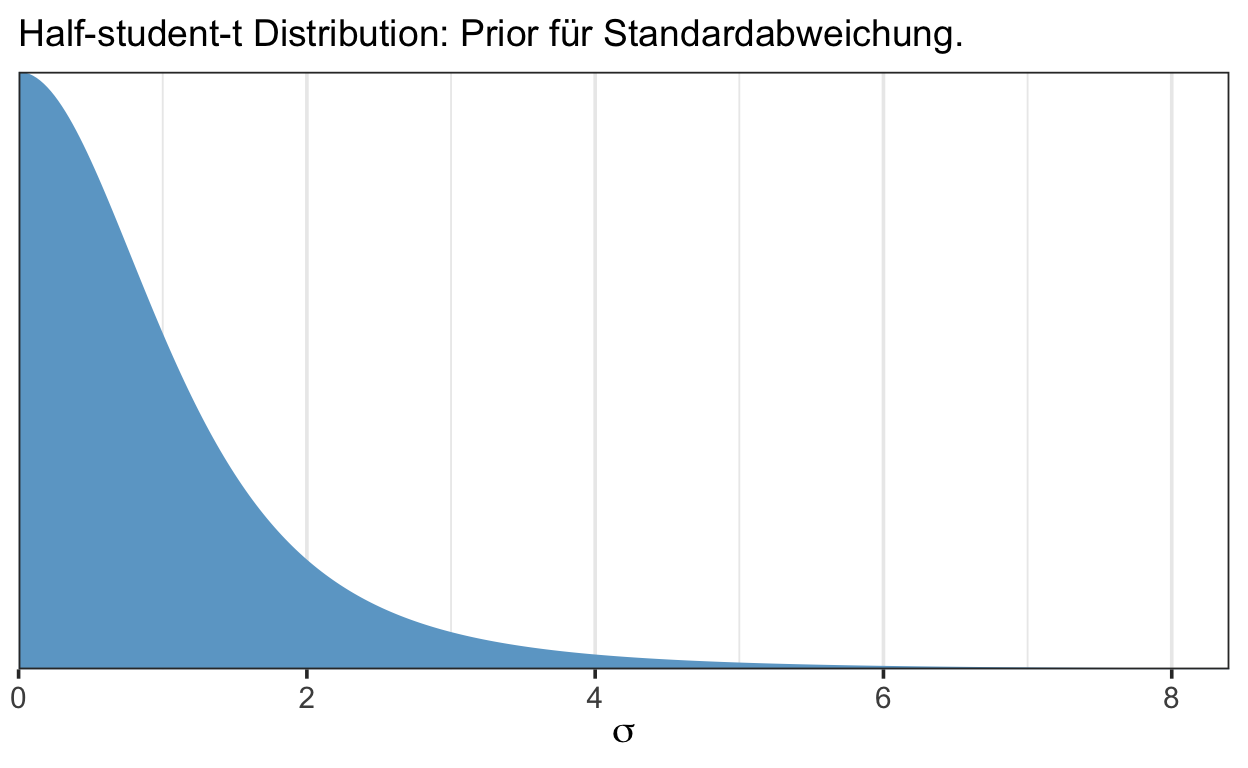
Figure 3: Prior für \(\sigma\).

Mittelwert

Für \(\mu\) erhalten wir ebenfalls eine t-Verteilung, student_t(3, 102, 3). Diese hat ebenfalls einen Normalitätsparameter \(\nu\) von 3, aber setzt die Location und Scale Parameter bei 102 und 3 (102 entspricht ungefähr dem Mittelwert). Grafik 4 yiegt diese Verteilung.

tibble(x = seq(from = 0, to = 200, by = .025)) %>% 
  mutate(d = dnorm(x, mean = 102, sd = 3)) %>% 
  ggplot(aes(x = x, ymin = 0, ymax = d)) +
  geom_ribbon(fill = "skyblue3") +
  scale_x_continuous(expand = expansion(mult = c(0, 0.05))) +
  scale_y_continuous(expand = expansion(mult = c(0, 0.05)), breaks = NULL) +
  coord_cartesian(xlim = c(50, 150),
                  ylim = c(0, 0.15)) +
  xlab(expression(mu)) +
  labs(subtitle = "Normalverteilter Prior für Mittelwert") +
  theme_bw(base_size = 14)

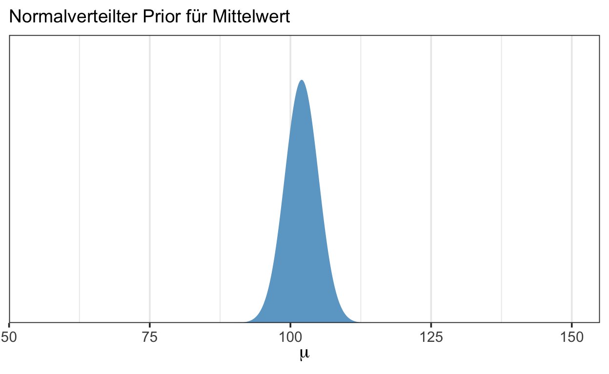
Figure 4: Prior für \(\mu\).

Prior Predictive Distribution

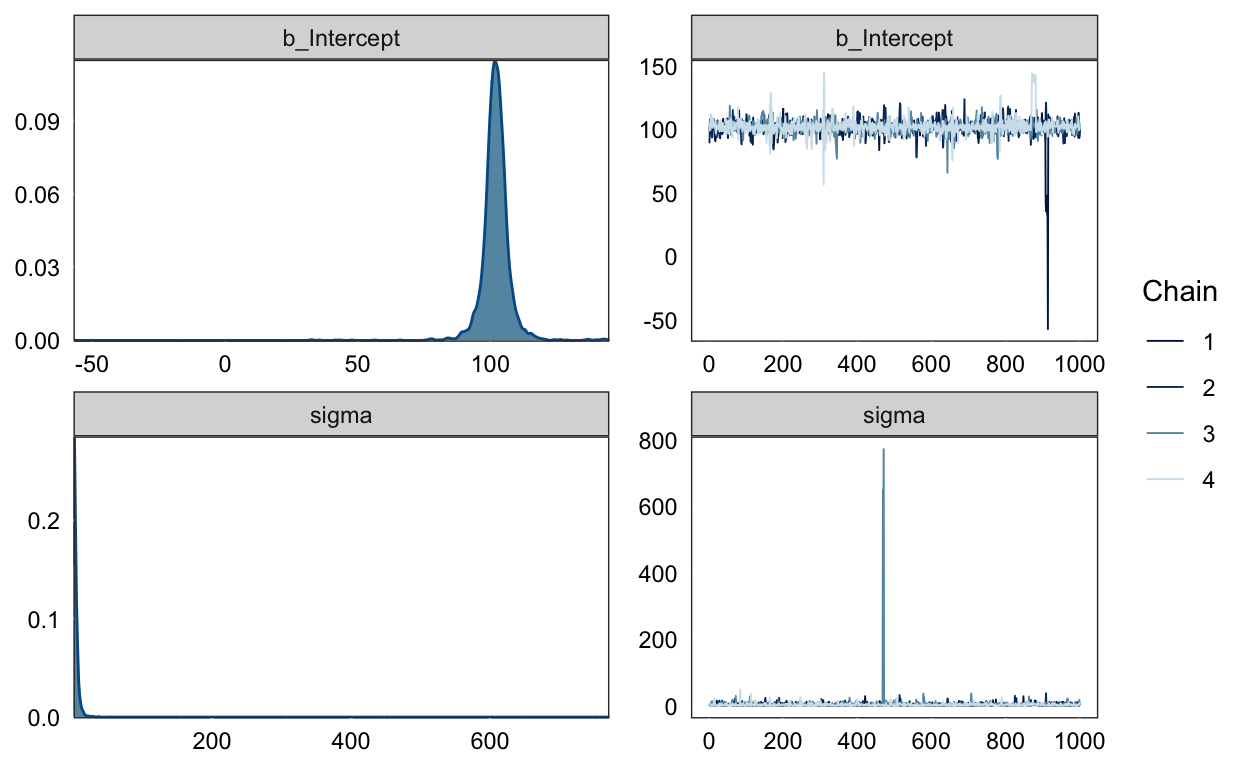
m1_prior <- brm(IQ ~ 1,
          prior = priors,
          data = d,
          sample_prior = "only",
          file = "models/twogroupiq-prior-1")

summary(m1_prior)

 Family: gaussian 
  Links: mu = identity; sigma = identity 
Formula: IQ ~ 1 
   Data: d (Number of observations: 47) 
Samples: 4 chains, each with iter = 2000; warmup = 1000; thin = 1;
         total post-warmup samples = 4000

Population-Level Effects: 
          Estimate Est.Error l-95% CI u-95% CI Rhat Bulk_ESS Tail_ESS
Intercept   101.95      6.20    92.34   111.71 1.00     2048     1510

Family Specific Parameters: 
      Estimate Est.Error l-95% CI u-95% CI Rhat Bulk_ESS Tail_ESS
sigma     3.75     17.71     0.10    12.94 1.00     1757     1199

Samples were drawn using sampling(NUTS). For each parameter, Bulk_ESS
and Tail_ESS are effective sample size measures, and Rhat is the potential
scale reduction factor on split chains (at convergence, Rhat = 1).

plot(m1_prior)

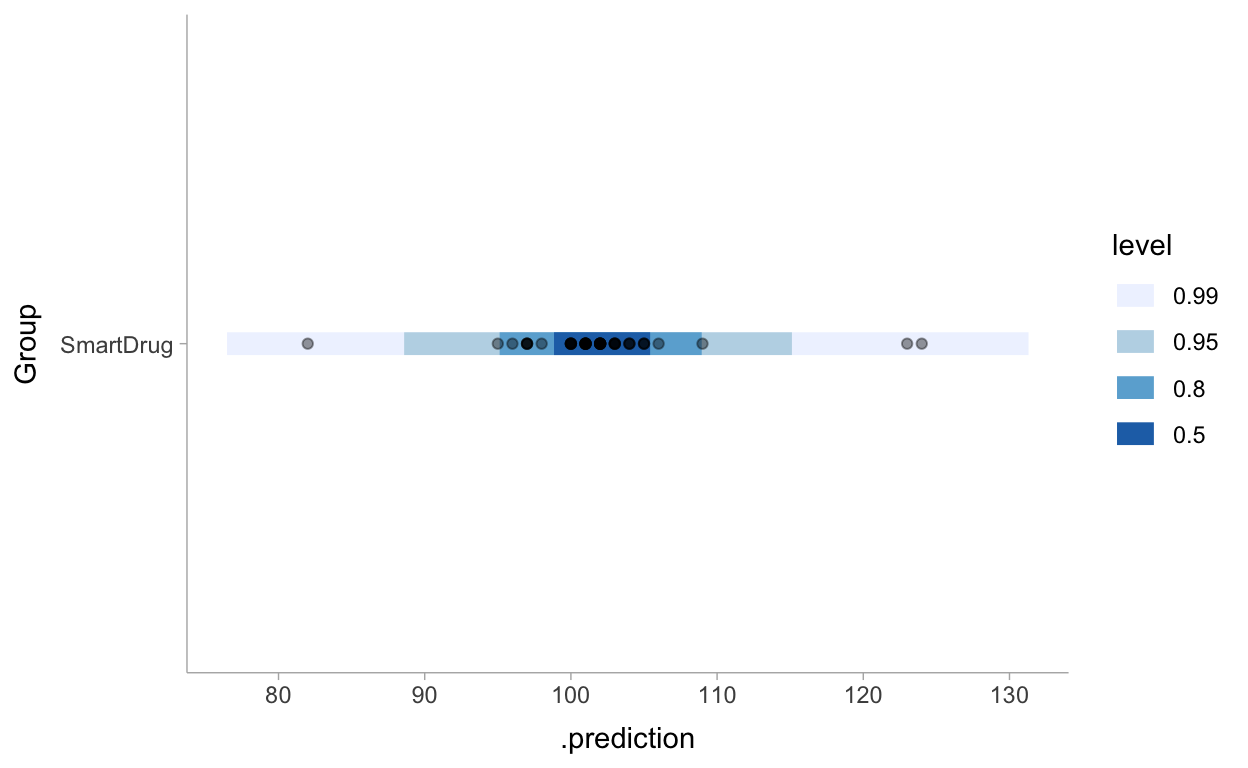
library(tidybayes)

prior_pred_1 <- d %>%
  modelr::data_grid(Group) %>%
  add_predicted_draws(m1_prior) %>%
  ggplot(aes(y = Group, x = .prediction)) +
  stat_interval(.width = c(.50, .80, .95, .99)) +
  geom_point(aes(x = IQ), alpha = 0.4,  data = d) +
  scale_color_brewer() +
  theme_tidybayes()

prior_pred_1

Die Posterior Verteilung durch Sampling approximieren

m1 <- brm(IQ ~ 1,
          prior = priors,
          data = d,
          file = "models/twogroupiq-1")

plot(m1)

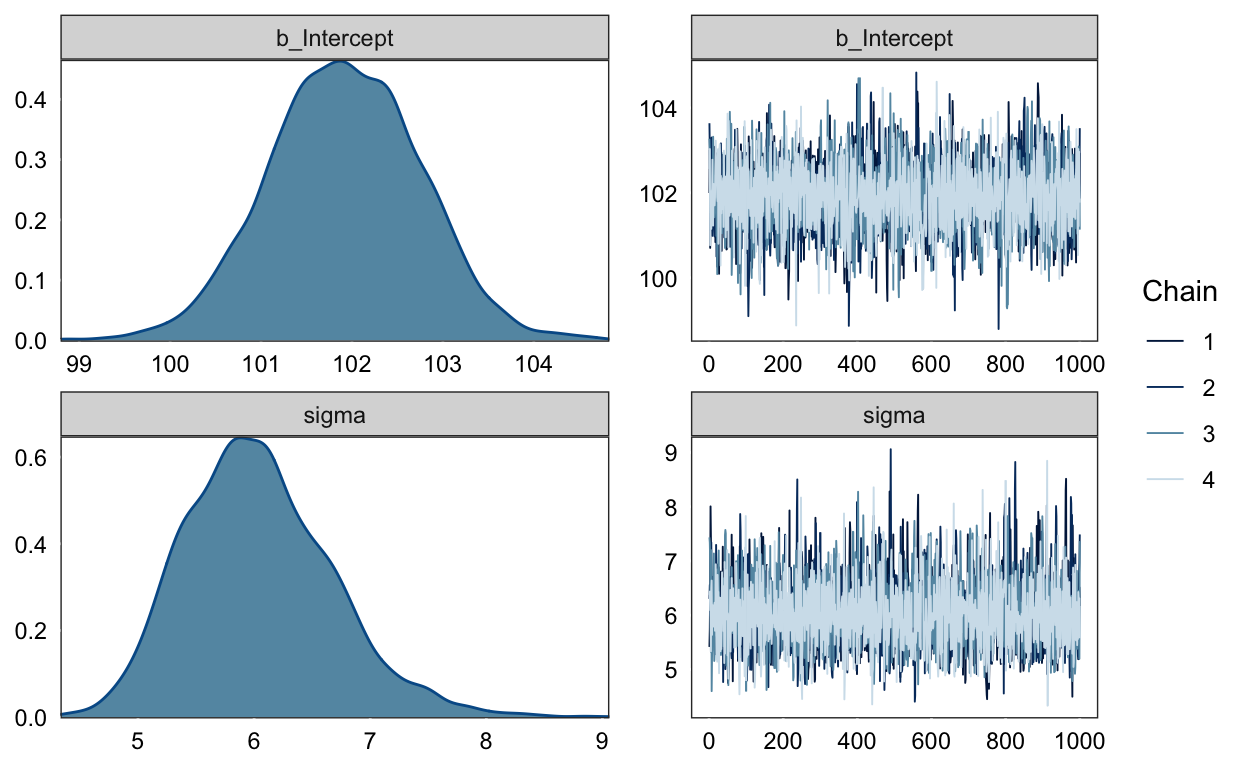
print(m1)

 Family: gaussian 
  Links: mu = identity; sigma = identity 
Formula: IQ ~ 1 
   Data: d (Number of observations: 47) 
Samples: 4 chains, each with iter = 2000; warmup = 1000; thin = 1;
         total post-warmup samples = 4000

Population-Level Effects: 
          Estimate Est.Error l-95% CI u-95% CI Rhat Bulk_ESS Tail_ESS
Intercept   101.92      0.83   100.31   103.53 1.00     3134     2075

Family Specific Parameters: 
      Estimate Est.Error l-95% CI u-95% CI Rhat Bulk_ESS Tail_ESS
sigma     6.04      0.64     4.96     7.47 1.00     3060     2458

Samples were drawn using sampling(NUTS). For each parameter, Bulk_ESS
and Tail_ESS are effective sample size measures, and Rhat is the potential
scale reduction factor on split chains (at convergence, Rhat = 1).

Posterior Quantile Intervals

mcmc_plot(m1, pars = "b_") 

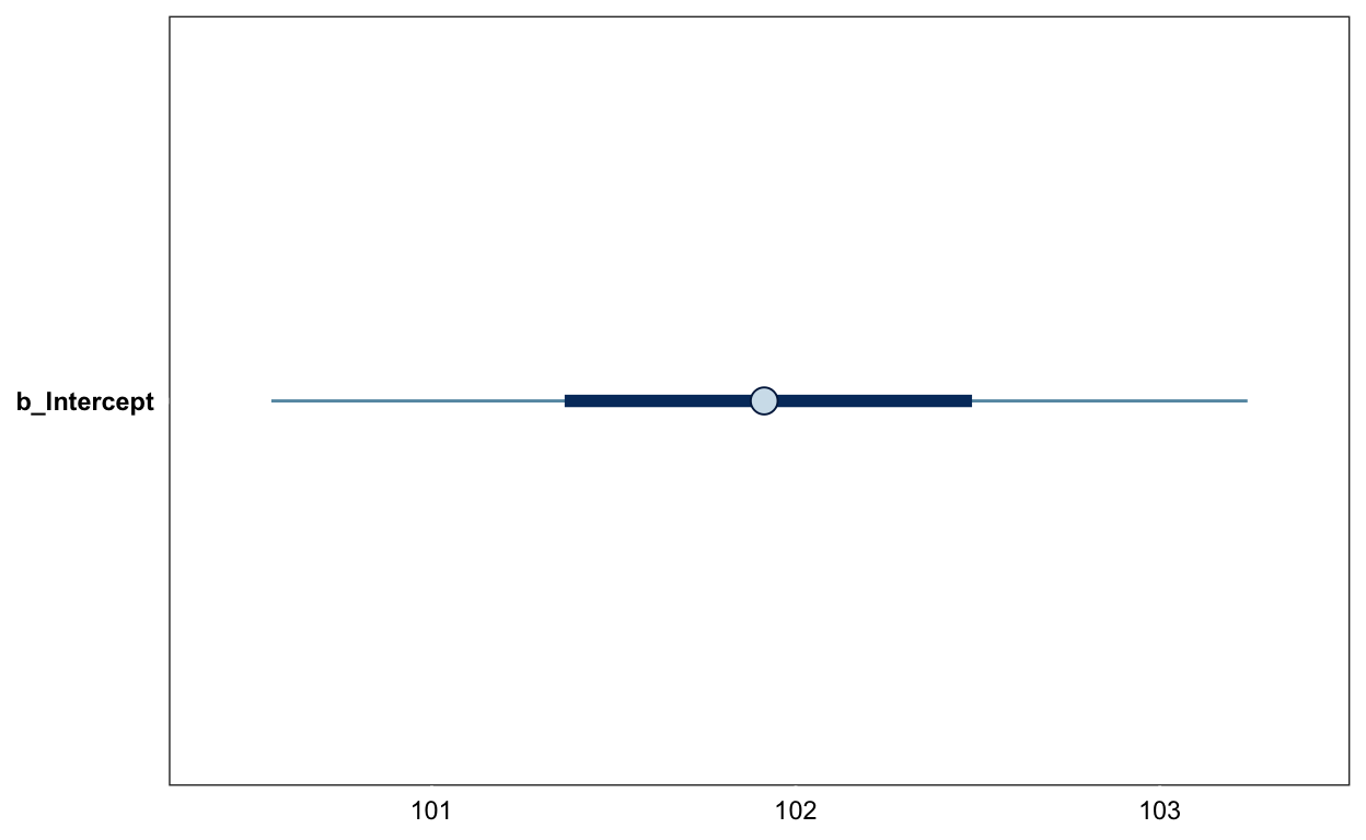
mcmc_plot(m1, pars = "sigma")

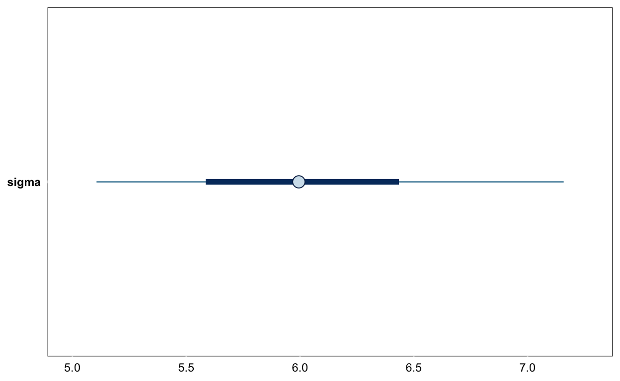
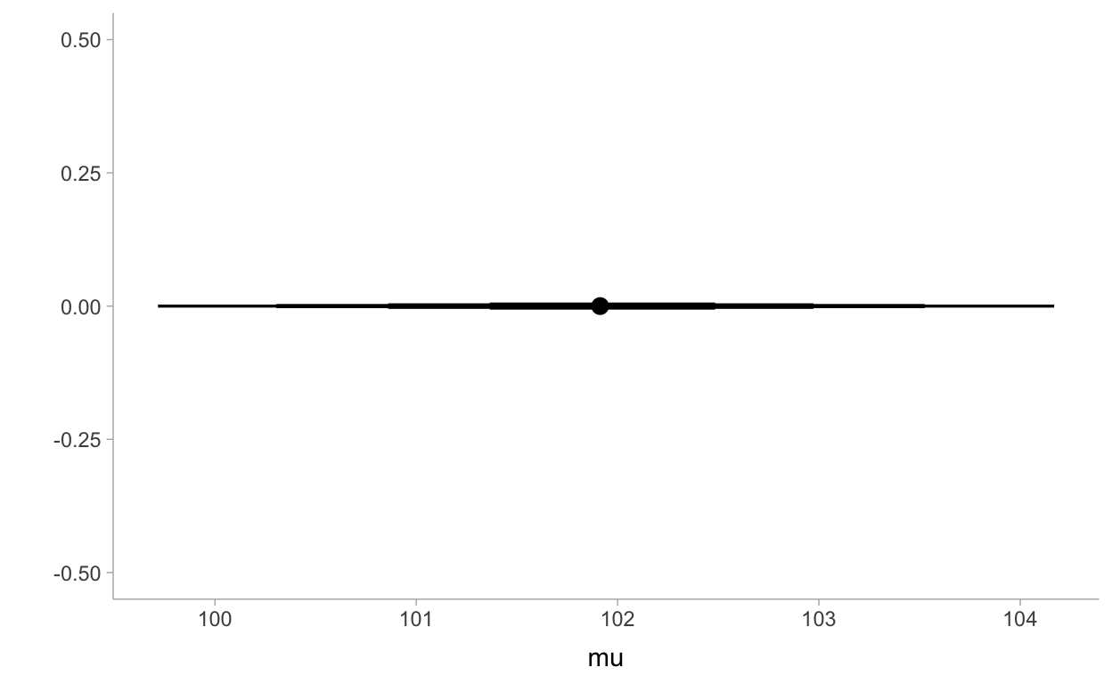
Posterior Samples extrahieren

samples <- posterior_samples(m1) %>% 
  transmute(mu = b_Intercept, sigma = sigma)

library(tidybayes)

samples %>% 
  select(mu) %>% 
  median_qi(.width = c(.50, .80, .95, .99))

        mu    .lower   .upper .width .point .interval
1 101.9132 101.36505 102.4841   0.50 median        qi
2 101.9132 100.86039 102.9730   0.80 median        qi
3 101.9132 100.30502 103.5255   0.95 median        qi
4 101.9132  99.71696 104.1686   0.99 median        qi

samples %>% 
  select(mu) %>% 
  median_qi(.width = c(.50, .80, .95, .99)) %>% 
  ggplot(aes(x = mu, xmin = .lower, xmax = .upper)) +
  geom_pointinterval() +
  ylab("") +
  theme_tidybayes()

samples %>% 
  select(mu) %>% 
  ggplot(aes(x = mu)) +
  stat_halfeye() +
  theme_tidybayes()

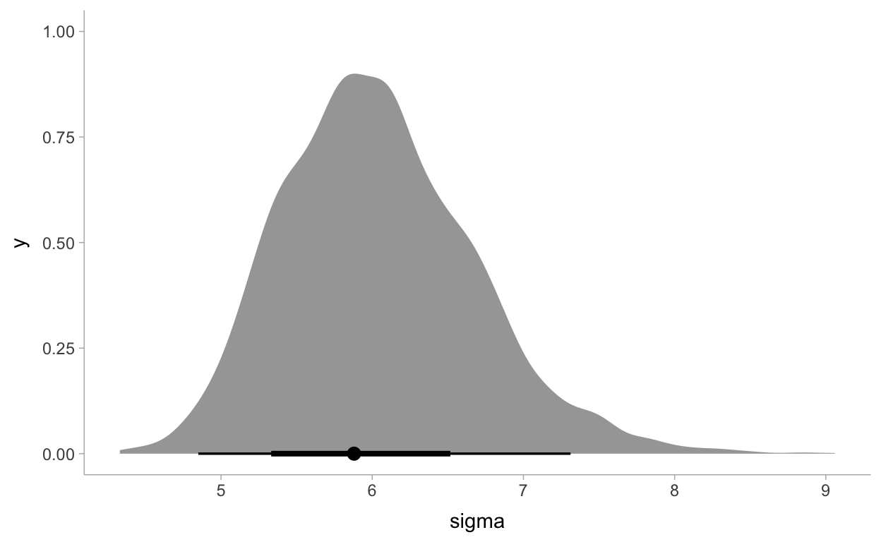
samples %>% 
  select(sigma) %>% 
  ggplot(aes(x = sigma)) +
  stat_halfeye(point_interval = mode_hdi) +
  theme_tidybayes()

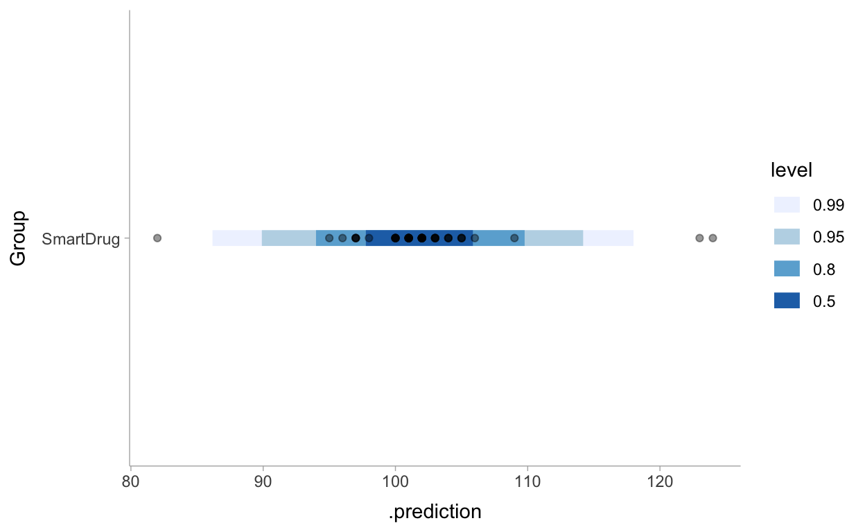
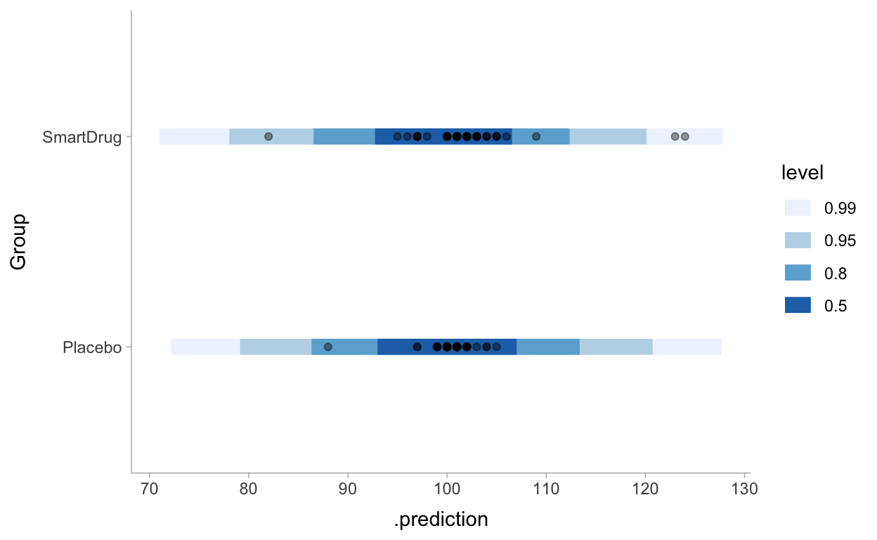
Posterior Predictive Distribution

post_pred_1 <- d %>%
  modelr::data_grid(Group) %>%
  add_predicted_draws(m1) %>%
  ggplot(aes(y = Group, x = .prediction)) +
  stat_interval(.width = c(.50, .80, .95, .99)) +
  geom_point(aes(x = IQ), alpha = 0.4,  data = d) +
  scale_color_brewer() +
  theme_tidybayes()

post_pred_1

Prior vs Posterior Predictive Distribution

# cowplot fall nötig installieren
if (!("cowplot" %in% installed.packages())) {install.packages("cowplot")}

cowplot::plot_grid(prior_pred_1, 
                   post_pred_1, 
                   labels = c('Prior predictive', 'Posterior predictive'), 
                   label_size = 12,
                   align = "h",
                   nrow = 2)

Zwei Gruppen

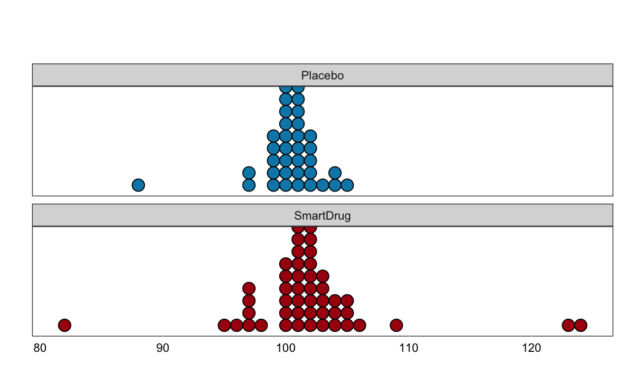
TwoGroupIQ %>%
   ggplot(aes(x = IQ, fill = Group)) +
      geom_dotplot(binwidth = 1) + 
      scale_fill_manual(values = c("#0288b7", "#a90010"), guide = FALSE) +
      scale_y_continuous(breaks = NULL) +
      labs(y = "Count", x = "IQ") +
      facet_wrap(~ Group, nrow = 2) +
      plot_annotation(title = "IQ difference",
                      subtitle = "Smart drug vs placebo",
                      theme = theme(plot.title = element_text(face = "bold",
                                                          size = rel(1.5))))

t-Test als Allgemeines Lineares Modell

Wir nehmen hier zunächst an, dass die beiden Gruppen dieselbe Varainz haben (Varianzgleichheit), obwohl wir vermuten, dass dies nicht der Fall ist.

Diese Annahme wäre nicht nötig; wir könnten problemlos für beide Gruppen eine eigene Standardabweichung schätzen.

Tradionelle Notation

\[y_{ij} = \alpha + \beta x_{ij} + \epsilon_{ij}\]

\[\epsilon \sim N(0, \sigma^2)\]

Probabilistische Notation

\[y_{ij} \sim N(\mu, \sigma^2)\] \[\mu_{ij} = \alpha + \beta x_{ij}\]

\(X_{ij}\) ist eine Indikatorvariable.

Ordinary Least Squares Schätzung

levels(TwoGroupIQ$Group)

[1] "Placebo"   "SmartDrug"

Mit R Formelnotation:

fit_ols <- lm(IQ ~ Group,
              data = TwoGroupIQ)

summary(fit_ols)

Call:
lm(formula = IQ ~ Group, data = TwoGroupIQ)

Residuals:
     Min       1Q   Median       3Q      Max 
-19.9149  -0.9149   0.0851   1.0851  22.0851 

Coefficients:
               Estimate Std. Error t value Pr(>|t|)    
(Intercept)    100.3571     0.7263 138.184   <2e-16 ***
GroupSmartDrug   1.5578     0.9994   1.559    0.123    
---
Signif. codes:  0 '***' 0.001 '**' 0.01 '*' 0.05 '.' 0.1 ' ' 1

Residual standard error: 4.707 on 87 degrees of freedom
Multiple R-squared:  0.02717,   Adjusted R-squared:  0.01599 
F-statistic:  2.43 on 1 and 87 DF,  p-value: 0.1227

Dummy Coding in R

contrasts(TwoGroupIQ$Group)

          SmartDrug
Placebo           0
SmartDrug         1

mm1 <- model.matrix(~ Group, data = TwoGroupIQ)
head(mm1)

  (Intercept) GroupSmartDrug
1           1              1
2           1              1
3           1              1
4           1              1
5           1              1
6           1              1

as_tibble(mm1) %>% 
  group_by(GroupSmartDrug) %>% 
  slice_sample(n= 3)

# A tibble: 6 x 2
# Groups:   GroupSmartDrug [2]
  `(Intercept)` GroupSmartDrug
          <dbl>          <dbl>
1             1              0
2             1              0
3             1              0
4             1              1
5             1              1
6             1              1

Dummy Coding in R

as_tibble(mm1) %>% 
  group_by(GroupSmartDrug) %>% 
  slice_sample(n= 3)

# A tibble: 6 x 2
# Groups:   GroupSmartDrug [2]
  `(Intercept)` GroupSmartDrug
          <dbl>          <dbl>
1             1              0
2             1              0
3             1              0
4             1              1
5             1              1
6             1              1

mm2 <- model.matrix(~ 0 + Group, data = TwoGroupIQ)
as_tibble(mm2) %>% 
  group_by(GroupSmartDrug) %>% 
  slice_sample(n= 3)

# A tibble: 6 x 2
# Groups:   GroupSmartDrug [2]
  GroupPlacebo GroupSmartDrug
         <dbl>          <dbl>
1            1              0
2            1              0
3            1              0
4            0              1
5            0              1
6            0              1

Graphical Model

Figure 5: Graphical Model für 2 Gruppen.

Get Priors

priors2 <- get_prior(IQ ~ 1 + Group,
                     data = TwoGroupIQ)

priors2

                  prior     class           coef group resp dpar
                 (flat)         b                               
                 (flat)         b GroupSmartDrug                
 student_t(3, 101, 2.5) Intercept                               
   student_t(3, 0, 2.5)     sigma                               
 nlpar bound       source
                  default
             (vectorized)
                  default
                  default

Get Priors

priors3 <- get_prior(IQ ~ 0 + Group,
                     data = TwoGroupIQ)

priors3

                prior class           coef group resp dpar nlpar
               (flat)     b                                     
               (flat)     b   GroupPlacebo                      
               (flat)     b GroupSmartDrug                      
 student_t(3, 0, 2.5) sigma                                     
 bound       source
            default
       (vectorized)
       (vectorized)
            default

Priors definieren und vom Prior Sampeln

priors2_b <- prior(normal(0, 2), class = b)

m2_prior <- brm(IQ ~ 1 + Group,
          prior = priors2_b,
          data = TwoGroupIQ,
          sample_prior = "only",
          file = "models/twogroupiq-prior-2")

prior_pred_2 <- TwoGroupIQ %>%
  modelr::data_grid(Group) %>%
  add_predicted_draws(m2_prior) %>%
  ggplot(aes(y = Group, x = .prediction)) +
  stat_interval(.width = c(.50, .80, .95, .99)) +
  geom_point(aes(x = IQ), alpha = 0.4,  data = TwoGroupIQ) +
  scale_color_brewer() +
  theme_tidybayes()

Priors definieren und vom Prior Sampeln

priors3_b <- prior(normal(100, 10), class = b)

m3_prior <- brm(IQ ~ 0 + Group,
          prior = priors3_b,
          data = TwoGroupIQ,
          sample_prior = "only",
          file = "models/twogroupiq-prior-3")

prior_pred_3 <- TwoGroupIQ %>%
  modelr::data_grid(Group) %>%
  add_predicted_draws(m3_prior) %>%
  ggplot(aes(y = Group, x = .prediction)) +
  stat_interval(.width = c(.50, .80, .95, .99)) +
  geom_point(aes(x = IQ), alpha = 0.4,  data = TwoGroupIQ) +
  scale_color_brewer() +
  theme_tidybayes()

Posterior Sampling

m2 <- brm(IQ ~ 1 + Group,
          prior = priors2_b,
          data = TwoGroupIQ,
          file = "models/twogroupiq-2")

m3 <- brm(IQ ~ 0 + Group,
          prior = priors3_b,
          data = TwoGroupIQ,
          file = "models/twogroupiq-3")

Summary

summary(m2)

 Family: gaussian 
  Links: mu = identity; sigma = identity 
Formula: IQ ~ 1 + Group 
   Data: TwoGroupIQ (Number of observations: 89) 
Samples: 4 chains, each with iter = 2000; warmup = 1000; thin = 1;
         total post-warmup samples = 4000

Population-Level Effects: 
               Estimate Est.Error l-95% CI u-95% CI Rhat Bulk_ESS
Intercept        100.51      0.69    99.18   101.90 1.00     3735
GroupSmartDrug     1.23      0.88    -0.49     2.95 1.00     3633
               Tail_ESS
Intercept          2921
GroupSmartDrug     3160

Family Specific Parameters: 
      Estimate Est.Error l-95% CI u-95% CI Rhat Bulk_ESS Tail_ESS
sigma     4.72      0.36     4.09     5.52 1.00     3002     2088

Samples were drawn using sampling(NUTS). For each parameter, Bulk_ESS
and Tail_ESS are effective sample size measures, and Rhat is the potential
scale reduction factor on split chains (at convergence, Rhat = 1).

Summary

summary(m3)

 Family: gaussian 
  Links: mu = identity; sigma = identity 
Formula: IQ ~ 0 + Group 
   Data: TwoGroupIQ (Number of observations: 89) 
Samples: 4 chains, each with iter = 2000; warmup = 1000; thin = 1;
         total post-warmup samples = 4000

Population-Level Effects: 
               Estimate Est.Error l-95% CI u-95% CI Rhat Bulk_ESS
GroupPlacebo     100.35      0.73    98.95   101.75 1.00     3914
GroupSmartDrug   101.92      0.69   100.62   103.28 1.00     4057
               Tail_ESS
GroupPlacebo       3163
GroupSmartDrug     2954

Family Specific Parameters: 
      Estimate Est.Error l-95% CI u-95% CI Rhat Bulk_ESS Tail_ESS
sigma     4.71      0.36     4.07     5.45 1.00     3342     2697

Samples were drawn using sampling(NUTS). For each parameter, Bulk_ESS
and Tail_ESS are effective sample size measures, and Rhat is the potential
scale reduction factor on split chains (at convergence, Rhat = 1).

mcmc_plot(m2, "b_GroupSmartDrug")

mcmc_plot(m3, "b")

Get Posterior Samples

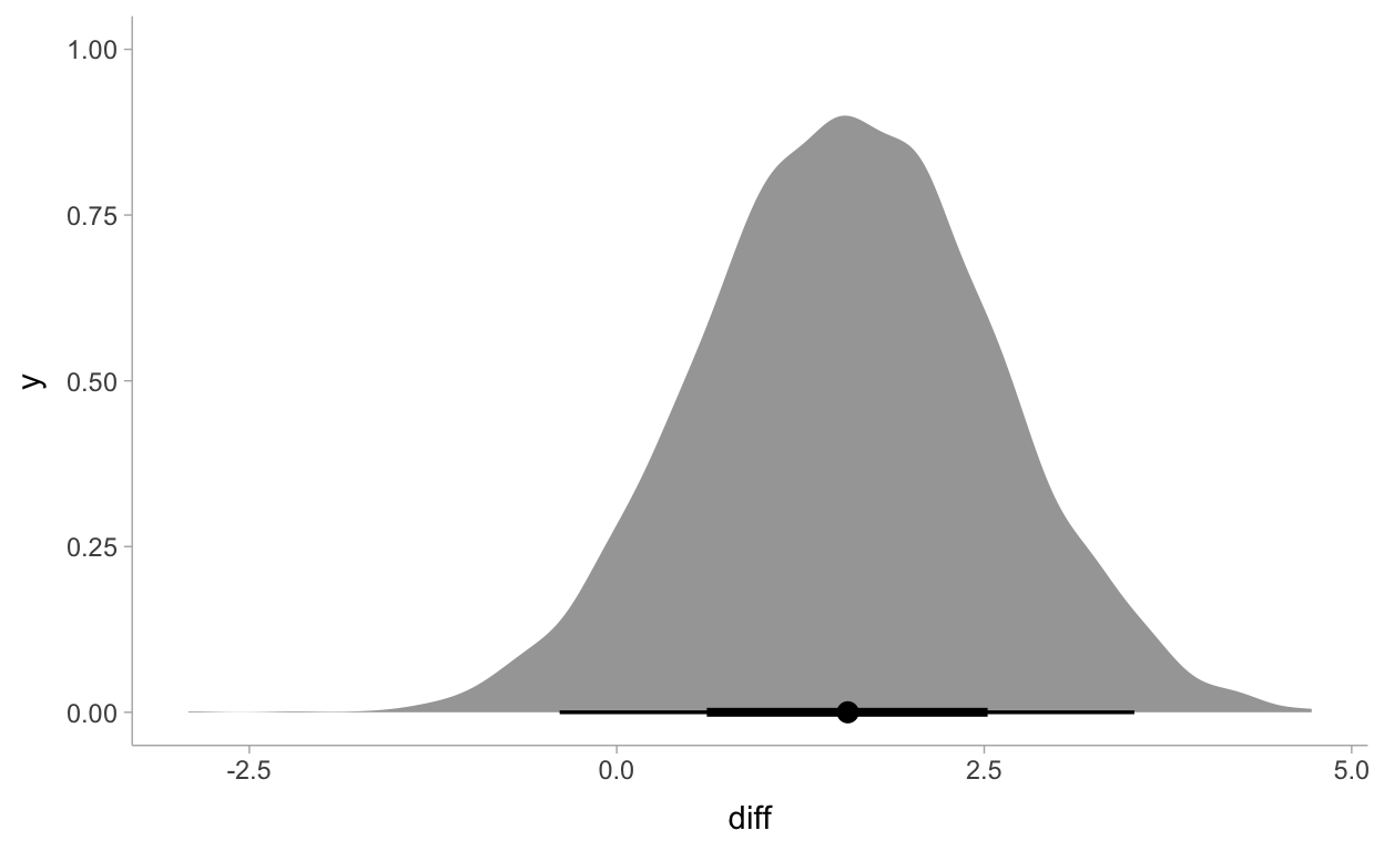
samples_m3 <- posterior_samples(m3) %>% 
    transmute(Placebo = b_GroupPlacebo, 
              SmartDrug = b_GroupSmartDrug,
              sigma = sigma)

samples_m3 <- samples_m3 %>% 
  mutate(diff = SmartDrug - Placebo,
         effect_size = diff/sigma)

Get Posterior Samples

samples_m3 %>% 
  select(diff) %>% 
  median_qi()

     diff     .lower   .upper .width .point .interval
1 1.57189 -0.3887631 3.521777   0.95 median        qi

samples_m3 %>% 
  select(diff) %>% 
  ggplot(aes(x = diff)) +
  stat_halfeye(point_interval = median_qi) +
  theme_tidybayes()

samples_m3 %>% 
  select(effect_size) %>% 
  ggplot(aes(x = effect_size)) +
  stat_halfeye(point_interval = median_qi) +
  theme_tidybayes()

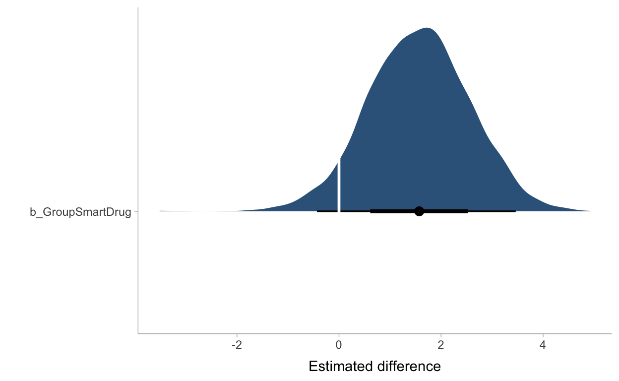
Diesmal ohne eigene Priors

fit_eqvar <- brm(IQ ~ Group,
                 data = TwoGroupIQ,
                 file = here::here("models/fit_eqvar"))

fit_eqvar %>%
    gather_draws(b_GroupSmartDrug) %>%
    ggplot(aes(y = .variable, x = .value)) +
    stat_halfeye(fill = "Steelblue4") +
    geom_vline(xintercept = 0, color = "white", linetype = 1, size = 1) +
    ylab("") +
    xlab("Estimated difference") +
    theme_tidybayes()

grid <- TwoGroupIQ %>%
    modelr::data_grid(Group)

fits_IQ <- grid %>%
    add_fitted_draws(fit_eqvar)

preds_IQ <- grid %>%
    add_predicted_draws(fit_eqvar)

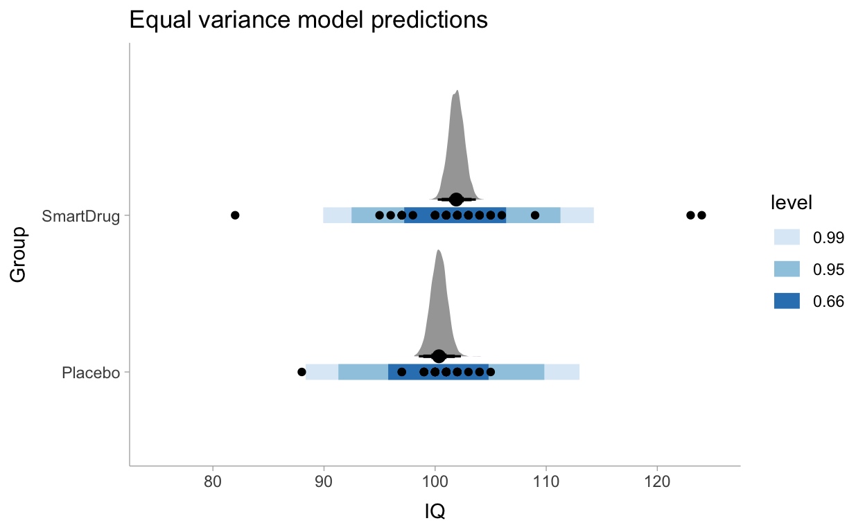
pp_eqvar <- TwoGroupIQ %>%
    ggplot(aes(x = IQ, y = Group)) +
    stat_halfeye(aes(x = .value),
                  scale = 0.7,
                  position = position_nudge(y = 0.1),
                  data = fits_IQ,
                  .width = c(.66, .95, 0.99)) +
    stat_interval(aes(x = .prediction),
                   data = preds_IQ,
                   .width = c(.66, .95, 0.99)) +
    scale_x_continuous(limits = c(75, 125)) +
    geom_point(data = TwoGroupIQ) +
    scale_color_brewer() +
  labs(title = "Equal variance model predictions") +
  theme_tidybayes()