Reaktionszeiten: I

Anwendungen.

Author

Affiliation

Andrew Ellis

Kognitive Psychologie, Wahrnehmung und Methodenlehre, Universität Bern

Published

2022-04-05

Note

👉 R Code für dieses Kapitel downloaden

👉 Daten downloaden

ADHD

library(tidyverse)

d <- read_csv("data/session-7.csv")

glimpse(d)

Rows: 300
Columns: 2
$ control <dbl> 700.2404, 1034.3323, 675.8451, 1027.1913, 781.4268, 637.8018, …
$ adhd    <dbl> 1457.7710, 736.0453, 1230.0827, 995.3828, 763.0127, 737.8560, …

d <- d |>
  pivot_longer(everything(), 
               names_to = "group", values_to = "rt") |> 
  mutate(group = as_factor(group)) |> 
  arrange(group)

glimpse(d)

Rows: 600
Columns: 2
$ group <fct> control, control, control, control, control, control, control, c…
$ rt    <dbl> 700.2404, 1034.3323, 675.8451, 1027.1913, 781.4268, 637.8018, 83…

p1 <- d |> 
  ggplot(aes(rt)) +
  geom_histogram(aes(y = ..density..), 
                 colour = "black", fill = "white",
                 binwidth = 10) +
  geom_density(lwd = 1, colour = 4,
               fill = 4, alpha = 0.25) +
  facet_wrap(~group, ncol = 1) +
  xlab("Response time [ms]") +
  xlim(c(0, 2200))

p1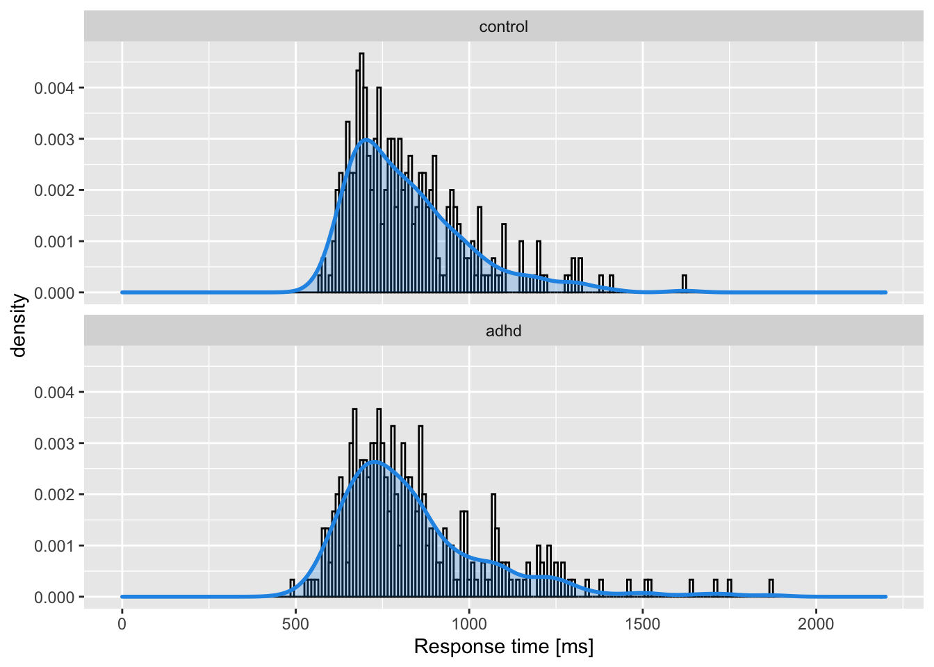

Zusammenfassen: zentrale Tendenz und Dispersion

Mittelwert und Standardabweichung

d %>% 
  group_by(group) %>% 
  summarise(mean = mean(rt),
            sd = sd(rt))

# A tibble: 2 × 3
  group    mean    sd
  <fct>   <dbl> <dbl>
1 control  822.  171.
2 adhd     839.  214.

Median und Interquartilsbereich

Der Interquartilsbereich repräntiert den Unterschied zwischen dem ersten (25. Perzentil) und dritten (75. Perzentil) Quartil. In diesem Bereich befinden sich 50% der Datenpunkte.

d %>% 
  group_by(group) %>% 
  summarise(mean = median(rt),
            q25 = quantile(rt, probs = 0.25),
            q75 = quantile(rt, probs = 0.75)) |> 
  mutate(IQR = q75 - q25)

# A tibble: 2 × 5
  group    mean   q25   q75   IQR
  <fct>   <dbl> <dbl> <dbl> <dbl>
1 control  782.  694.  898.  205.
2 adhd     784.  694.  923.  228.

d %>% 
  group_by(group) %>% 
  summarise(mean = median(rt),
            IQR = IQR(rt))

# A tibble: 2 × 3
  group    mean   IQR
  <fct>   <dbl> <dbl>
1 control  782.  205.
2 adhd     784.  228.

funs <- list(mean = mean, median = median, 
             sd = sd, IQR = IQR)

by_group <- d |>
  group_by(group) |>
  summarise(across(rt, funs, .names = "{.fn}")) |>
  mutate(across(where(is.numeric), ~round(., 2)))

by_group

# A tibble: 2 × 5
  group    mean median    sd   IQR
  <fct>   <dbl>  <dbl> <dbl> <dbl>
1 control  822.   782.  171.  205.
2 adhd     839.   784.  214.  228.

p1 +
  geom_vline(aes(xintercept = mean), 
             data = by_group,
             color = "steelblue",
             lwd = 1.5) +
  geom_vline(aes(xintercept = median), 
             data = by_group, 
             color = "red",
             lwd = 1.5)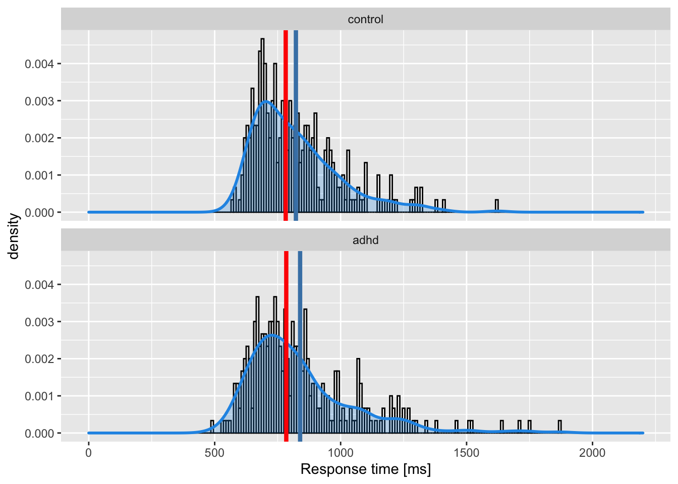

Zentrale Tendenz bei schiefen Verteilungen

Sowohl Mittelwert als auch Median sind jedoch problematisch als Masse der zentralen Tendenz für asymmetrische Verteilungen. Der Mittelwert kann durch eine hohe Schiefe und Ausreissern verschoben werden, und repräsentiert die zentrale Tendenz der Verteilung nicht besonders gut.

Der Median ist ein besseres Mass für eine typische Beobachtung aus dieser Verteilung, ist jedoch nicht erwartungstreu, das heisst der Median überschätzt den Populationsmedian. Der Grad der Überschätzung steigt mit sinkender Anzahl Beobachtungen (d.h. vor allem bei kleinen Stichproben).

Quantile

deciles <- seq(0.1, 0.9, length.out = 9)

quantile_fun <- function(x, probs = c(0.25, 0.5, 0.75)) {
  tibble(rt = quantile(x, probs, type = 8), quantile = probs)
}

d_quantiles <- d %>% 
  group_by(group) %>% 
  summarise(quantile_fun(rt, probs = deciles))

d_quantiles

# A tibble: 18 × 3
# Groups:   group [2]
   group      rt quantile
   <fct>   <dbl>    <dbl>
 1 control  649.      0.1
 2 control  684.      0.2
 3 control  711.      0.3
 4 control  740.      0.4
 5 control  782.      0.5
 6 control  826.      0.6
 7 control  875.      0.7
 8 control  949.      0.8
 9 control 1045.      0.9
10 adhd     631.      0.1
11 adhd     674.      0.2
12 adhd     712.      0.3
13 adhd     745.      0.4
14 adhd     784.      0.5
15 adhd     828.      0.6
16 adhd     874.      0.7
17 adhd     980.      0.8
18 adhd    1108.      0.9

Shift function

Wir müssen nun den Dataframe mit den Quantilen ins “wide” Format konvertieren, um zwei Spalten für die control und adhd Gruppen zu erhalten. Danach können wir die Differenzen zwischen den Gruppen für jedes Quantil berechnen.

d_quantile_differences <- d_quantiles |> 
  pivot_wider(names_from = "group", values_from = "rt")

d_quantile_differences

# A tibble: 9 × 3
  quantile control  adhd
     <dbl>   <dbl> <dbl>
1      0.1    649.  631.
2      0.2    684.  674.
3      0.3    711.  712.
4      0.4    740.  745.
5      0.5    782.  784.
6      0.6    826.  828.
7      0.7    875.  874.
8      0.8    949.  980.
9      0.9   1045. 1108.

d_quantile_differences <- d_quantile_differences |> 
    mutate(`control - adhd` = control - adhd)

d_quantile_differences

# A tibble: 9 × 4
  quantile control  adhd `control - adhd`
     <dbl>   <dbl> <dbl>            <dbl>
1      0.1    649.  631.            18.2 
2      0.2    684.  674.            10.6 
3      0.3    711.  712.            -1.45
4      0.4    740.  745.            -4.99
5      0.5    782.  784.            -2.16
6      0.6    826.  828.            -1.57
7      0.7    875.  874.             1.42
8      0.8    949.  980.           -30.4 
9      0.9   1045. 1108.           -62.8

Shift function grafisch darstellen

d_quantile_differences %>% 
  ggplot(aes(x = control, y = `control - adhd`)) +
  geom_hline(yintercept = 0, linetype = 3) +
  geom_vline(xintercept = d_quantile_differences %>% 
               filter(quantile == "50%") %>% 
               select(adhd) %>% 
               pull(), linetype = 3) +
  geom_line(aes(group = 1), color = "steelblue", size = 2) +
  geom_point(shape = 21, color = "steelblue", fill = "white", size = 5, stroke = 1) +
  coord_cartesian(ylim = c(-300, 300))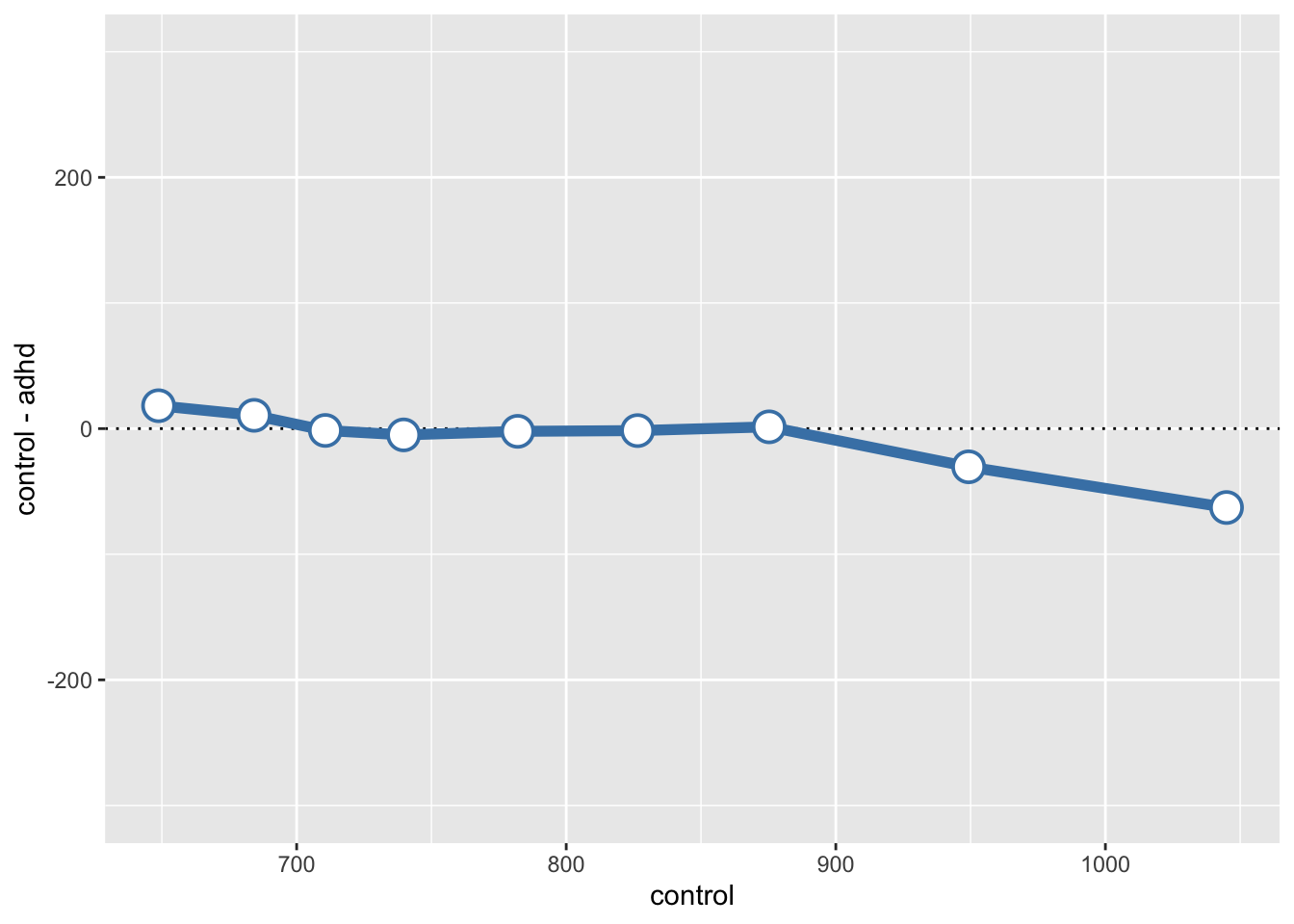

install.packages("remotes")
remotes::install_github("GRousselet/rogme")

# library(rogme)

out <- rogme::shifthd(d, rt ~ group)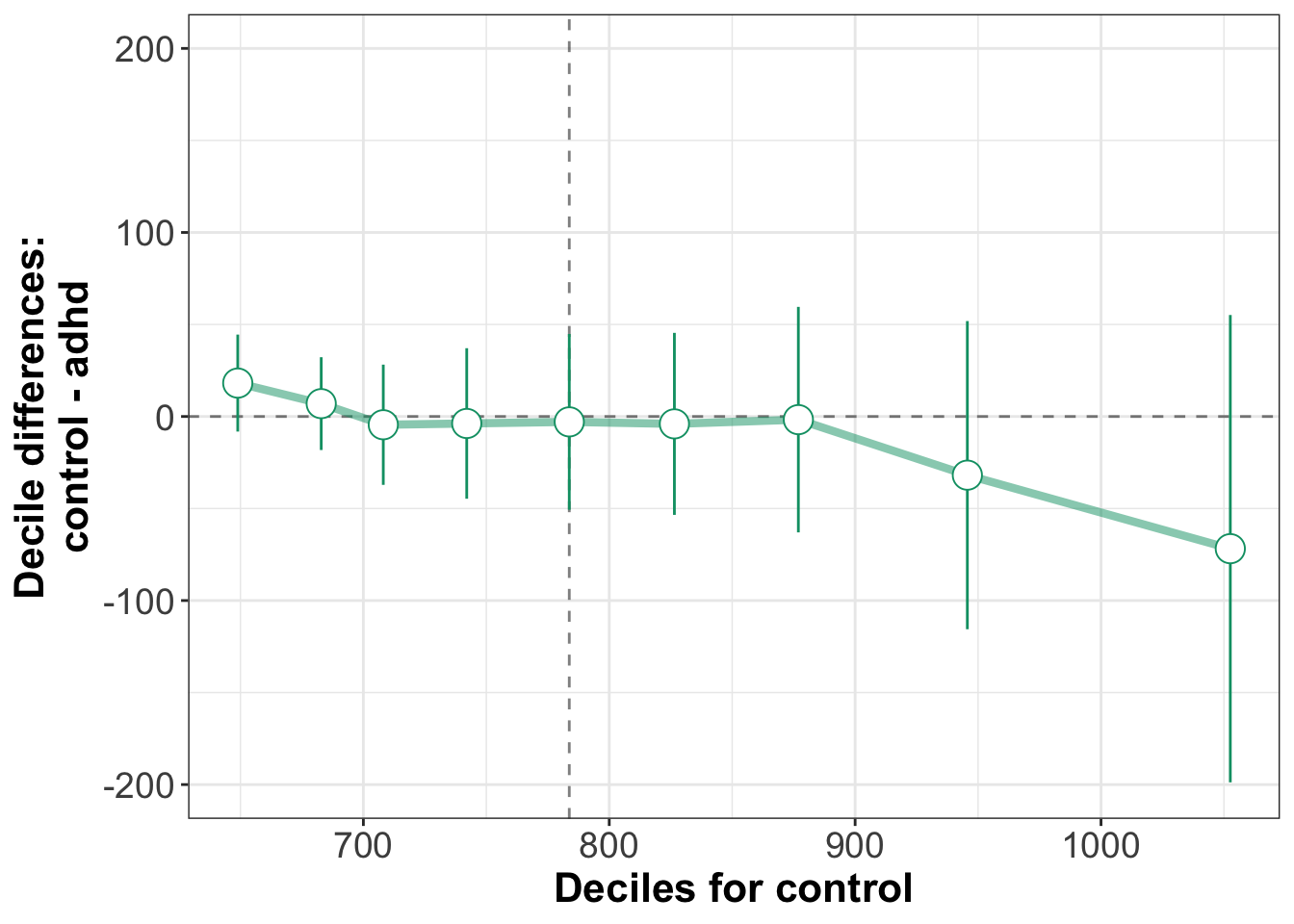

rogme::plot_sf(out)

[[1]]

Reuse

https://creativecommons.org/licenses/by/4.0/

Citation

BibTeX citation:

@online{ellis2022,
  author = {Andrew Ellis},
  title = {Reaktionszeiten: {I}},
  date = {2022-04-05},
  url = {https://kogpsy.github.io/neuroscicomplabFS22//pages/chapters/07_response_times_i.html},
  langid = {en}
}

For attribution, please cite this work as:

Andrew Ellis. 2022. “Reaktionszeiten: I.” April 5, 2022. https://kogpsy.github.io/neuroscicomplabFS22//pages/chapters/07_response_times_i.html.