8. Sitzung
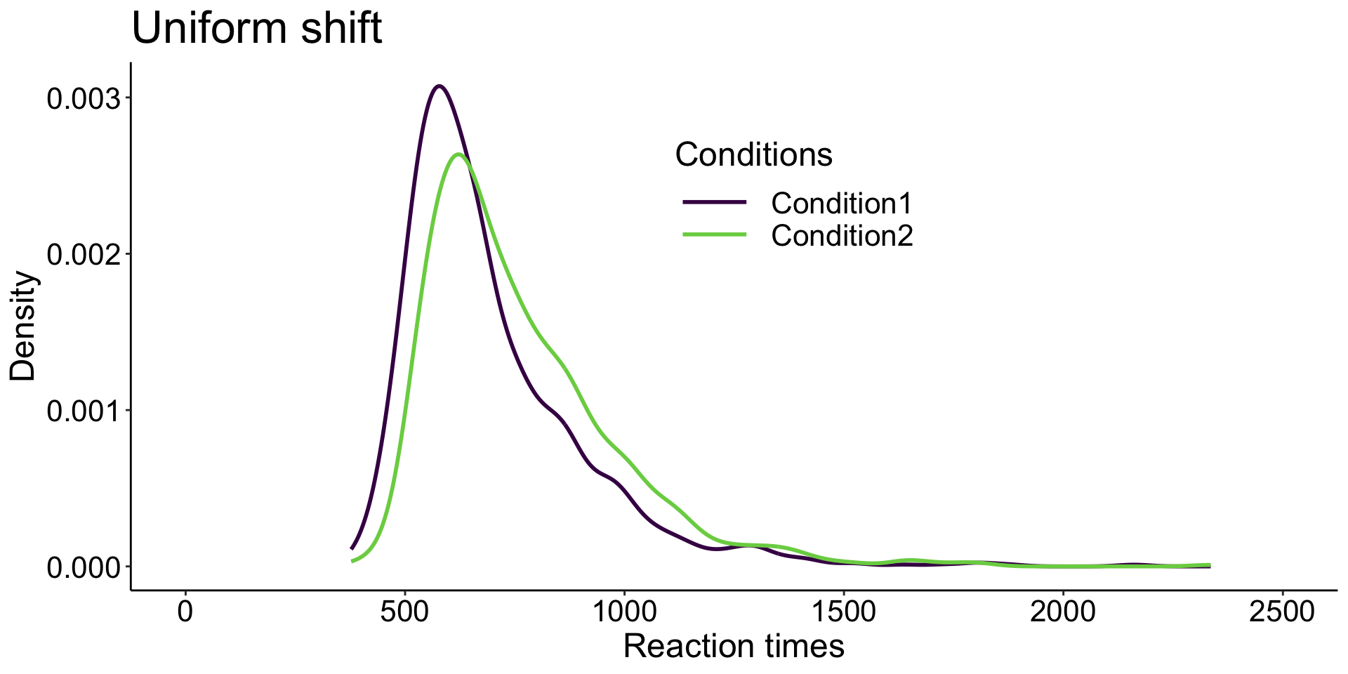
Response Times
Neurowissenschaft Computerlab FS 22
2022-04-12
Experimental manipulations
affects most strongly slow behavioural responses, but with limited effects on fast responses.
affects all responses, fast and slow, similarly.
has stronger effects on fast responses, and weaker ones for slow responses.
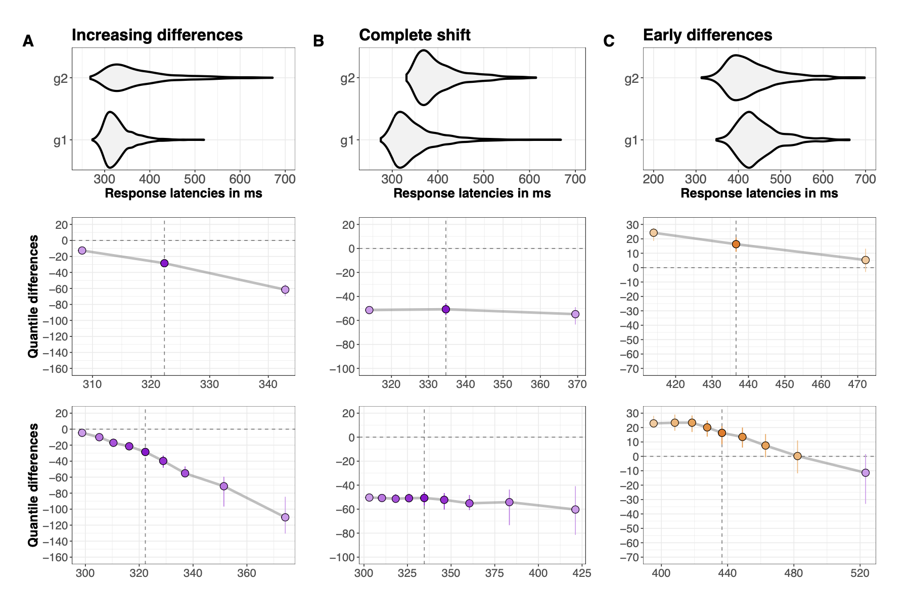
Distribution analysis provides much stronger constraints on the underlying cognitive architecture than comparisons limited to e.g. mean or median reaction times across participants.
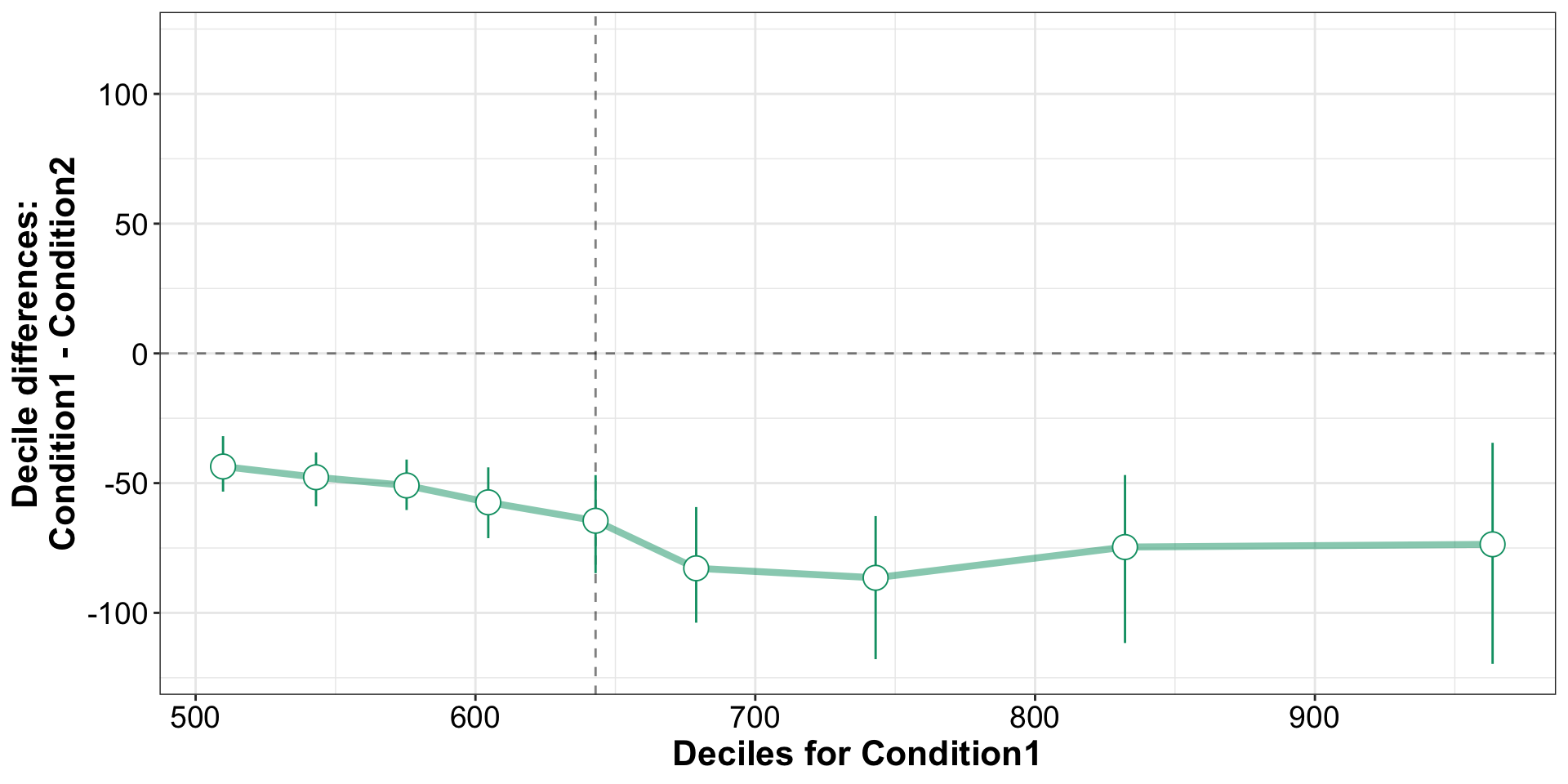
Shift Function: Independent Groups
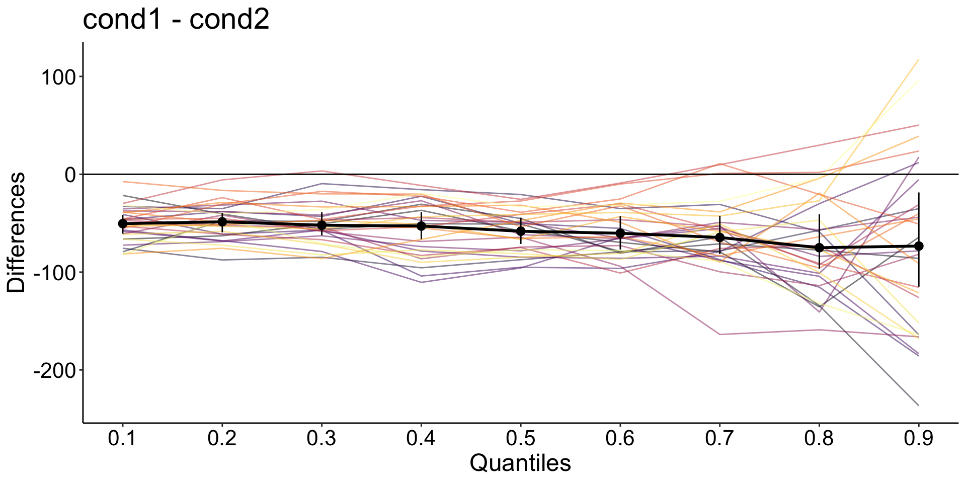
Hierarchical Shift Function

Participants with all quantile differences > 0
nq <- length(out$quantiles)
pdmt0 <- apply(out$individual_sf > 0, 2, sum)
print(paste0('In ',sum(pdmt0 == nq),' participants (',round(100 * sum(pdmt0 == nq) / np, digits = 1),'%), all quantile differences are more than to zero'))
[1] "In 0 participants (0%), all quantile differences are more than to zero"Participants with all quantile differences < 0
Hierarchical Shift Function
Alternative bootstrapping method: hsf_pb()
Bootstrapping
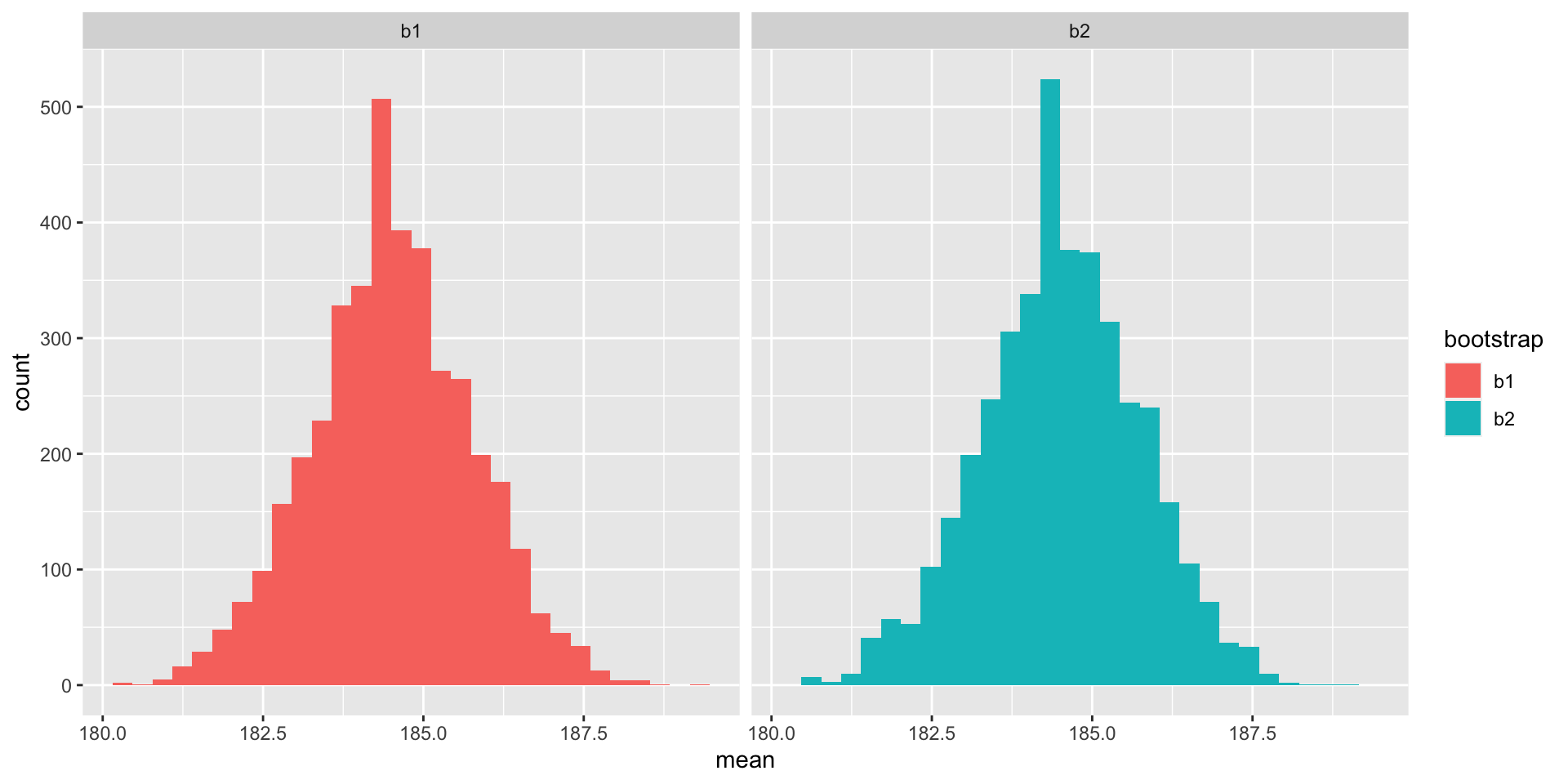
Bootstrapping
Bootstrapped standard error of the mean: