Signal Detection Theory: II

Beispiel: PsychoPy Experiment.

Author

Affiliation

Andrew Ellis

Kognitive Psychologie, Wahrnehmung und Methodenlehre, Universität Bern

Published

2022-03-29

Note

👉 R Code für dieses Kapitel downloaden

👉 Daten downloaden

SDT Kennzahlen für alle VPn berechnen

Wir werden nun d', k und c (bias) für alle Versuchspersonen in diesem Datensatz berechnen.

Note

Wichtig: Was erwarten wir für die Parameter d' und c? Hinweis: Der Cue war entweder rechts oder links (oder neutral). Wie sollte das die Parameter beeinflussen?

Daten importieren

Zuerst die Daten downloaden, und speichern.

library(tidyverse)
d <- read_csv("data/session-6.csv")

Variablen bearbeiten

Zu factor konvertieren, etc.

d <- d |>
    select(ID, condition, cue, direction, choice) |>
    mutate(across(where(is.character), ~as_factor(.)),
           cue = fct_relevel(cue, "left", "none", "right")) |>
    drop_na()

Trials klassifizieren

Als Hit, Miss, CR und FA.

sdt <- d |>
    mutate(type = case_when(
        direction == "___" & choice == "___" ~ "___"),
        ___,
        ___,
        ___)

sdt

# A tibble: 2,362 × 6
   ID     condition cue   direction choice type 
   <fct>  <fct>     <fct> <fct>     <fct>  <chr>
 1 chch04 valid     left  left      left   CR   
 2 chch04 valid     left  left      left   CR   
 3 chch04 valid     left  left      right  FA   
 4 chch04 invalid   right left      left   CR   
 5 chch04 neutral   none  left      left   CR   
 6 chch04 valid     left  left      left   CR   
 7 chch04 invalid   right left      left   CR   
 8 chch04 valid     left  left      left   CR   
 9 chch04 neutral   none  left      left   CR   
10 chch04 neutral   none  right     left   Miss 
# … with 2,352 more rows

SDT Kennzahlen zusammenzählen

sdt_summary <- sdt |>
    group_by(ID, cue) |>
    count(type)

sdt_summary

# A tibble: 170 × 4
# Groups:   ID, cue [45]
   ID     cue   type      n
   <fct>  <fct> <chr> <int>
 1 chch04 left  CR       29
 2 chch04 left  FA        3
 3 chch04 left  Hit       7
 4 chch04 left  Miss      1
 5 chch04 none  CR       38
 6 chch04 none  FA        2
 7 chch04 none  Hit      34
 8 chch04 none  Miss      6
 9 chch04 right CR        5
10 chch04 right FA        3
# … with 160 more rows

Von `wide` zu `long` konvertieren

sdt_summary <- sdt_summary |>
    pivot_wider(names_from = type, values_from = n)

sdt_summary

# A tibble: 45 × 6
# Groups:   ID, cue [45]
   ID     cue      CR    FA   Hit  Miss
   <fct>  <fct> <int> <int> <int> <int>
 1 chch04 left     29     3     7     1
 2 chch04 none     38     2    34     6
 3 chch04 right     5     3    25     7
 4 chmi14 left     21    10     5     3
 5 chmi14 none     18    19    29     7
 6 chmi14 right     3     4    26     4
 7 J      left     19    12     5     3
 8 J      none     23    16    33     6
 9 J      right     6     2    20    12
10 jh     left     32    NA     5     3
# … with 35 more rows

Funktionen definieren

replace_NA <- function(x) {
    x = ifelse(is.na(x), 0, x)
    x
}

correct_zero_one <- function(x) {
    if (identical(x, 0)) {
        x = x + 0.001
    } else if (identical(x, 1)) {
        x = x - 0.001
    }
    x
}

NAs ersetzen

sdt_summary <- sdt_summary |>
    mutate(across(c(Hit, Miss, FA, CR), replace_NA))

Hit Rate und False Alarm Rate berechnen

sdt_summary <- sdt_summary |>
    mutate(hit_rate = ___,
           fa_rate = ___)

Werte 0 und 1 korrigieren

sdt_summary <- sdt_summary |>
    mutate(across(c(hit_rate, fa_rate), correct_zero_one))

Z-Transformation

sdt_summary <- sdt_summary |>
    mutate(zhr = ___,
           zfa = ___)

SDT Kennzahlen berechnen

sdt_summary <- sdt_summary |>
    mutate(dprime = ___,
           k = ___,
           c = ___) |>
    mutate(across(c(dprime, k, c), round, 2))

Variablen auswählen

sdt_final <- sdt_summary |>
    select(ID, cue, dprime, k, c)

SDT als GLM

Tip

Vertiefung: Wir können d', k und c auch als Regressionskoeffizienten einer Probit Regression schätzen.

Eine Person auswählen.

SU6460 <- d |>
    filter(ID %in% "SU6460")

SU6460_sdt <- sdt_final |>
    filter(ID %in% "SU6460")

Visualisieren

SU6460_sdt

# A tibble: 3 × 5
# Groups:   ID, cue [3]
  ID     cue   dprime     k     c
  <fct>  <fct>  <dbl> <dbl> <dbl>
1 SU6460 left    0.32  0    -0.16
2 SU6460 none    0.3  -0.23 -0.38
3 SU6460 right  -0.27 -0.67 -0.54

SU6460_sdt |>
    ggplot(aes(x = cue, y = dprime, group = 1)) +
    geom_line() +
    geom_point(shape = 21, size = 3, fill = "white")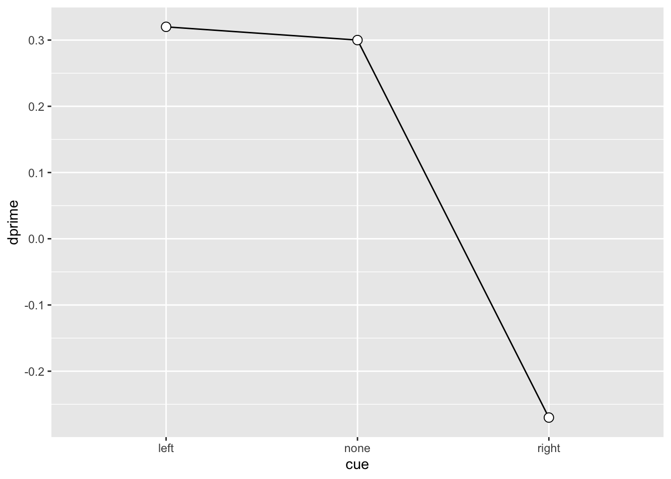

SU6460_sdt |>
    ggplot(aes(x = cue, y = c, group = 1)) +
    geom_line() +
    geom_point(shape = 21, size = 3, fill = "white")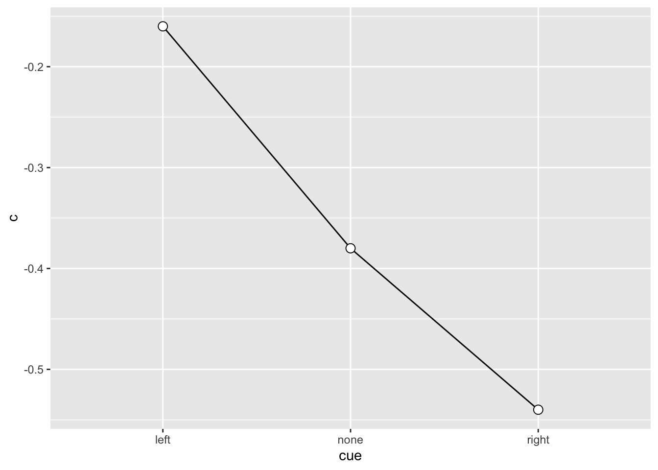

Generalized Linear Model

Check levels: right muss die zweite Faktorstufe sein!

levels(SU6460$choice)

[1] "left"  "right"

SU6460_glm_k_left <- glm(choice ~ direction,
                      family = binomial(link = "probit"),
                      data = SU6460 |> filter(cue == "left"))

summary(SU6460_glm_k_left)


Call:
glm(formula = choice ~ direction, family = binomial(link = "probit"), 
    data = filter(SU6460, cue == "left"))

Deviance Residuals: 
    Min       1Q   Median       3Q      Max  
-1.4006  -1.1774   0.9695   1.1774   1.1774  

Coefficients:
                 Estimate Std. Error z value Pr(>|z|)
(Intercept)    -1.250e-16  2.216e-01   0.000    1.000
directionright  3.186e-01  5.028e-01   0.634    0.526

(Dispersion parameter for binomial family taken to be 1)

    Null deviance: 55.352  on 39  degrees of freedom
Residual deviance: 54.946  on 38  degrees of freedom
AIC: 58.946

Number of Fisher Scoring iterations: 4

SU6460_glm_k_right <- glm(choice ~ direction,
                       family = binomial(link = "probit"),
                       data = SU6460 |> filter(cue == "right"))

summary(SU6460_glm_k_right)


Call:
glm(formula = choice ~ direction, family = binomial(link = "probit"), 
    data = filter(SU6460, cue == "right"))

Deviance Residuals: 
    Min       1Q   Median       3Q      Max  
-1.6651  -1.4614   0.9178   0.9178   0.9178  

Coefficients:
               Estimate Std. Error z value Pr(>|z|)
(Intercept)      0.6745     0.4818   1.400    0.162
directionright  -0.2722     0.5331  -0.511    0.610

(Dispersion parameter for binomial family taken to be 1)

    Null deviance: 50.446  on 39  degrees of freedom
Residual deviance: 50.181  on 38  degrees of freedom
AIC: 54.181

Number of Fisher Scoring iterations: 4

SU6460 <- SU6460 |>
    mutate(dir = if_else(direction == "left", -1/2, 1/2))

SU6460_glm_c_left <- glm(choice ~ dir,
                       family = binomial(link = "probit"),
                       data = SU6460 |> filter(cue == "left"))
summary(SU6460_glm_c_left)


Call:
glm(formula = choice ~ dir, family = binomial(link = "probit"), 
    data = filter(SU6460, cue == "left"))

Deviance Residuals: 
    Min       1Q   Median       3Q      Max  
-1.4006  -1.1774   0.9695   1.1774   1.1774  

Coefficients:
            Estimate Std. Error z value Pr(>|z|)
(Intercept)   0.1593     0.2514   0.634    0.526
dir           0.3186     0.5028   0.634    0.526

(Dispersion parameter for binomial family taken to be 1)

    Null deviance: 55.352  on 39  degrees of freedom
Residual deviance: 54.946  on 38  degrees of freedom
AIC: 58.946

Number of Fisher Scoring iterations: 4

SU6460_glm_c_right <- glm(choice ~ dir,
                        family = binomial(link = "probit"),
                        data = SU6460 |> filter(cue == "right"))

summary(SU6460_glm_c_right)


Call:
glm(formula = choice ~ dir, family = binomial(link = "probit"), 
    data = filter(SU6460, cue == "right"))

Deviance Residuals: 
    Min       1Q   Median       3Q      Max  
-1.6651  -1.4614   0.9178   0.9178   0.9178  

Coefficients:
            Estimate Std. Error z value Pr(>|z|)  
(Intercept)   0.5384     0.2665   2.020   0.0434 *
dir          -0.2722     0.5331  -0.511   0.6096  
---
Signif. codes:  0 '***' 0.001 '**' 0.01 '*' 0.05 '.' 0.1 ' ' 1

(Dispersion parameter for binomial family taken to be 1)

    Null deviance: 50.446  on 39  degrees of freedom
Residual deviance: 50.181  on 38  degrees of freedom
AIC: 54.181

Number of Fisher Scoring iterations: 4

Reuse

https://creativecommons.org/licenses/by/4.0/

Citation

BibTeX citation:

@online{ellis2022,
  author = {Andrew Ellis},
  title = {Signal {Detection} {Theory:} {II}},
  date = {2022-03-29},
  url = {https://kogpsy.github.io/neuroscicomplabFS22//pages/chapters/06_signal_detection_ii.html},
  langid = {en}
}

For attribution, please cite this work as:

Andrew Ellis. 2022. “Signal Detection Theory: II.” March 29, 2022. https://kogpsy.github.io/neuroscicomplabFS22//pages/chapters/06_signal_detection_ii.html.

SDT Kennzahlen für alle VPn berechnen

Daten importieren

Variablen bearbeiten

Trials klassifizieren

SDT Kennzahlen zusammenzählen

Von wide zu long konvertieren

Funktionen definieren

NAs ersetzen

Hit Rate und False Alarm Rate berechnen

Werte 0 und 1 korrigieren

Z-Transformation

SDT Kennzahlen berechnen

Variablen auswählen

SDT als GLM

Eine Person auswählen.

Visualisieren

Generalized Linear Model

Reuse

Citation

Von `wide` zu `long` konvertieren