In dieser Übung analysieren Sie Verhaltensdaten einer Studie, in welcher der Einfluss der kortikalen Aktivität im medial orbitofrontal cortex (mOFC) bei einer Konfliktsituation auf die Geschwindigkeit nachfolgender Antworten untersucht wurde (Verstynen 2014). Ein Konflikt wurde mittels eines colour-word Stroop Tasks induziert. Der Hauptbefund in Bezug auf die behavioralen Daten:
In a conflict-related region of the medial orbitofrontal cortex (mOFC), stronger BOLD responses predicted faster response times (RTs) on the next trial.
Stroop Task
Der durchgeführe Task ist eine Standardversion eines Stroop Tasks:
Stroop task. Participants performed the color-word version of the Stroop task (Botvinick et al. 2001; Gratton et al. 1992; Macleod 1991; Stroop 1935) comprised of congruent, incongruent, and neutral conditions while in the MR scanner. Participants were instructed to ignore the meaning of the printed word and respond to the ink color in which the word was printed. For example, in the congruent condition the words “RED,” “GREEN,” and “BLUE” were displayed in the ink colors red, green, and blue, respectively. In this condition, attentional demands were low because the ink color matched the prepotent response of reading the word, so response conflict was at a minimum. However, for the incongruent condition the printed words were different from the ink color in which they were printed (e.g., the word “RED” printed in blue ink). This condition elicited conflict because responding according to the printed word would result in an incorrect response. As a result, attentional demands were high and participants needed to inhibit the prepotent response of reading the word and respond according to the ink color in which the word was printed. On the other hand, the neutral condition consisted of noncolor words presented in an ink color (e.g., the word “CHAIR” printed in red ink) and had a low level of conflict and low attentional demands.
Versuchspersonen musste mit einer Response Box eine von drei Tasten drücken. Es wurde festgehalten, ob die Antwort korrekt war.
Participants were instructed to respond to the ink color in which the text appeared by pressing buttons under the index, middle, and ring fingers on their right hand, each button corresponding to one of the three colors (red, green, and blue, respectively) on an MR-safe response box. The task was briefly practiced in the scanner to acquaint the participant with the task and to ensure understanding of the instructions. The task began with the presentation of a fixation cross hair for 1,000 ms followed by the Stroop stimulus for 2,000 ms, during which participants were instructed to respond as quickly as possible. A total of 120 trials were presented to each participant (42 congruent, 42 neutral, 36 incongruent). A lower number of incongruent trials was used in order to reduce the expectancy of a stimulus conflict relative to the other conditions.
Datenanalyse
Von Interesse sind die Reaktionszeiten der korrekten Antworten in den Bedingungen kongruent, inkongruent und neutral.
Behavioral analysis. The primary behavioral variable of interest was response time (RT), recorded as the time between cue onset and registered key press (in milliseconds). All first-level analyses were restricted to correct responses. To determine condition-level effects, a one-way repeated-measures ANOVA was used, as were post hoc one-sample t-tests.
Rows: 3337 Columns: 4
── Column specification ────────────────────────────────────────────────────────
Delimiter: ","
chr (3): ID, condition, correct
dbl (1): RT

ℹ Use `spec()` to retrieve the full column specification for this data.
ℹ Specify the column types or set `show_col_types = FALSE` to quiet this message.
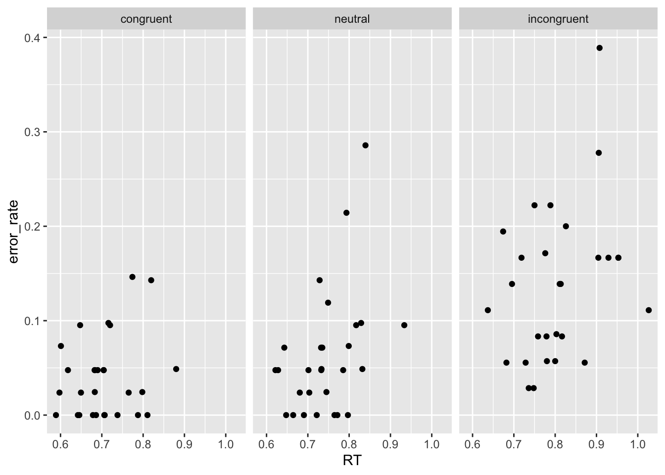
Es sieht aus, als sei die Fehlerrate im Mittel in der inkongruenten Bedingung grösser als in den kongruenten neutralen Bedingungen. Dies ist zu erwarten.
Wir wollen hier nur die Reaktionszeiten korrekter Antworten analysieren. Filtern Sie den Datensatz, so dass nur noch die korrekten Antworten bleiben.
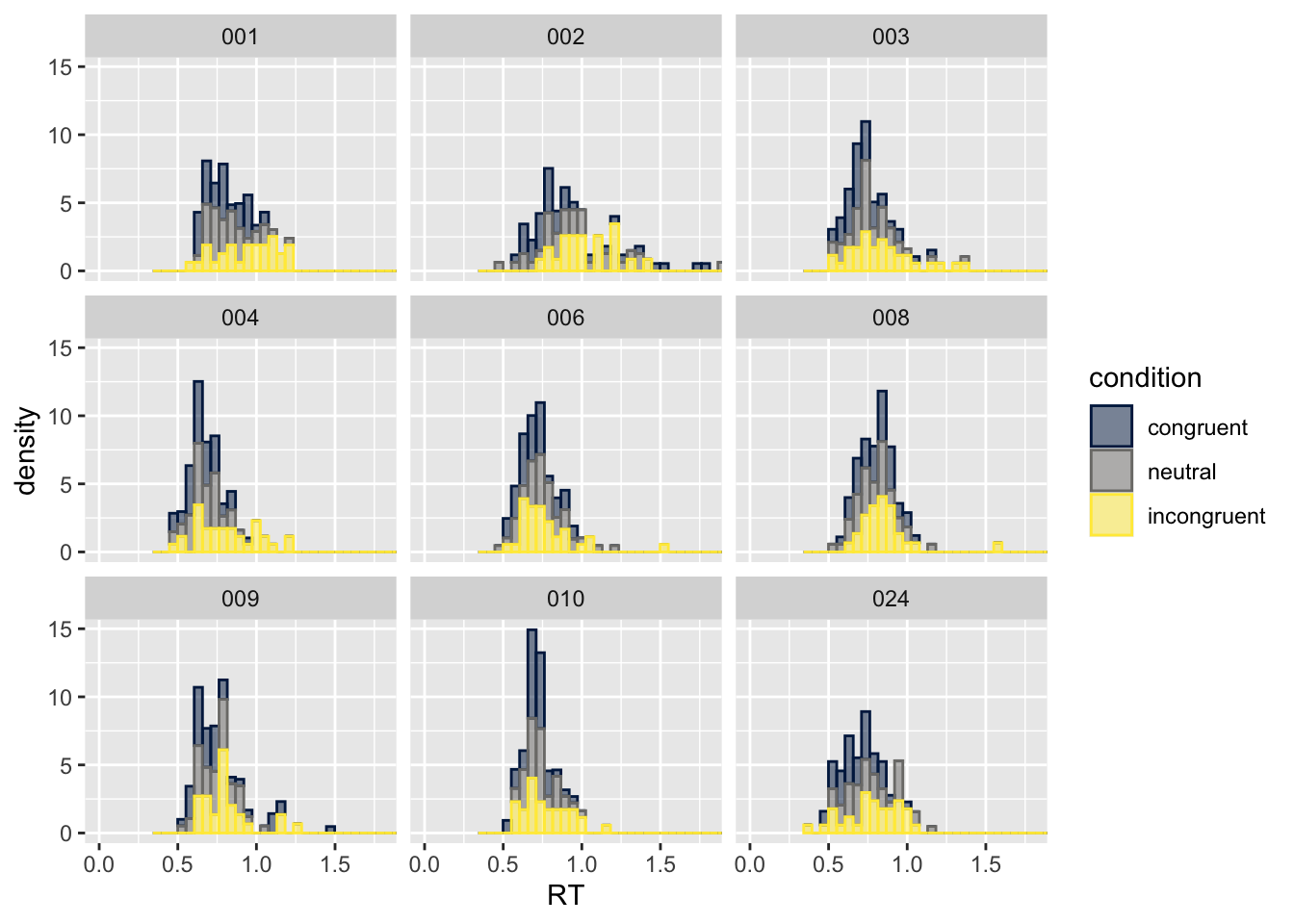
Wir plotten hier die RT Histogramme 9 zufällig ausgewählter Personen. ::: {.cell hash=‘solution_05_cache/html/unnamed-chunk-12_9b5124d7154035b458f8566b2b0ef58b’}
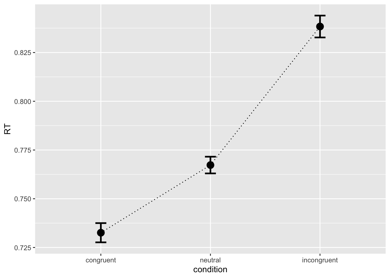
Berechnen Sie die mittlere RT pro Person/Bedingung, und stellen Sie die mittlere RT pro Bedingung, gemittelt über Personen, mit Fehlerbalken grafisch dar.
Beschreiben Sie in 1-2 Sätzen, was Sie gefunden haben.
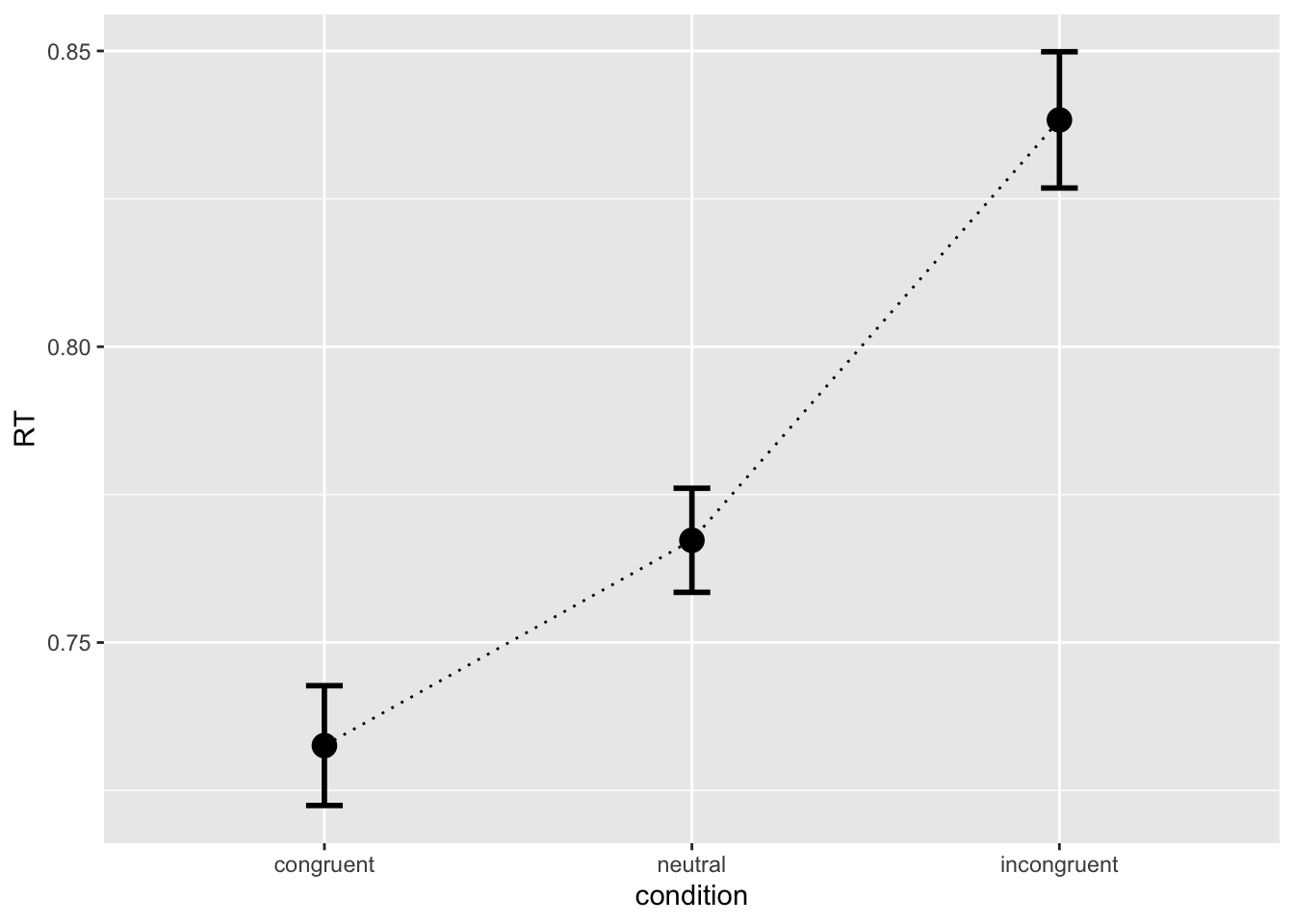
Die mittlere Reaktionszeit für korrekte Entscheidungen ist in der inkongruenten Bedingung grösser als in der neutralen Bedingungen, währens die mittlere RT in der kongruenten Bedingung kleiner als in der neutralen Bedingung. Wenn wir anstelle der Standardfehler die Konfidenzintervalle plotten, sehen wir, dass diese Unterschiede signifikant wären, wenn wir dies testen wollten (die 95% Konfidenzintervalle überlappen nicht).
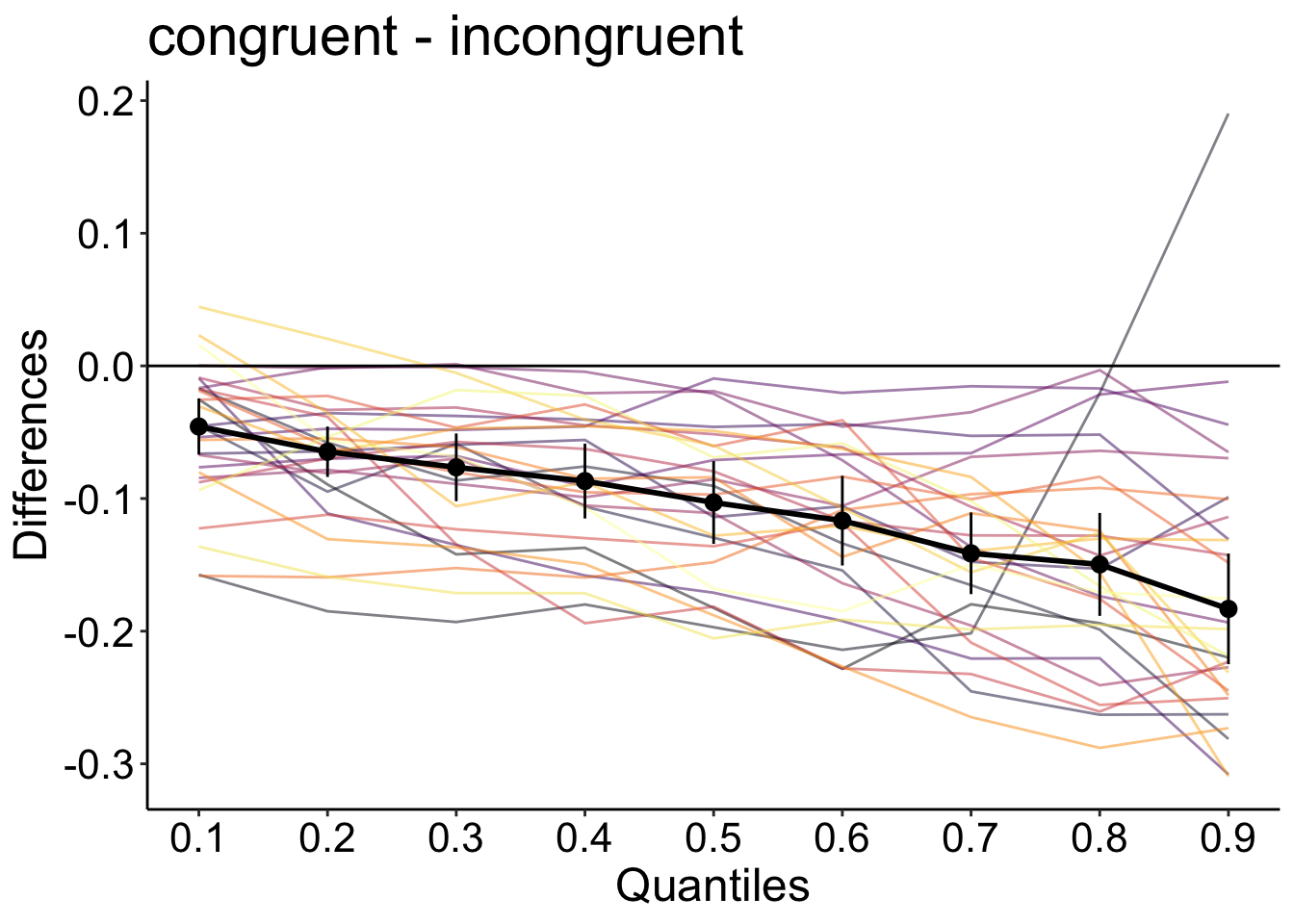
Nun verwenden wir die Funktion hsf() aus dem rogme Package, um Shift Functions für jede Person in den beiden Bedingungen zu berechnen, und die gemittelten Differenzen der Dezile zu erhalten.
Die Formel, welche Sie für die Funktion brauchen, lautet
RT~condition+ID
Diese Formel ist so zu lesen: RT Quantile werden durch condition und ID vorhergesagt.
Auf der X-Achse sind die Dezile der congruent Bedingung und auf der Y-Achse die Differenz congruent - incongruent. Die Differenz ist bei jedem Dezil negativ und scheint stetig stärker negativ zu werden. Die incongruent Bedingung führt zu längeren und variableren Reaktionszeiten. Der Stroop-Effekt, das heisst längere RTs bei inkongruenten Trials, ist bei langsamen Antworten stärker ausgeprägt. Dies ist mit dem Befund von Pratte et al. (2010) vereinbar.
References
Pratte, Michael S., Jeffrey N. Rouder, Richard D. Morey, and Chuning Feng. 2010. “Exploring the Differences in Distributional Properties Between Stroop and Simon Effects Using Delta Plots.”Attention, Perception, & Psychophysics 72 (7): 2013–25. https://doi.org/10.3758/APP.72.7.2013.
Verstynen, Timothy D. 2014. “The Organization and Dynamics of Corticostriatal Pathways Link the Medial Orbitofrontal Cortex to Future Behavioral Responses.”Journal of Neurophysiology 112 (10): 2457–69. https://doi.org/10.1152/jn.00221.2014.