Evidence Accumulation Models: II
Fitting models to data

Fitting models to data: Parameter estimation
The goal of fitting a model to data is to find the best-fitting parameter values. In other words, we want to find parameters of the model for which the probability of observing the data is maximized. i.e. we want to estimate parameters from the data. This is done by minimizing the error between the model’s predictions and the data.
Here, we will look at maximum likelihood estimation (MLE). The likelihood function is a function that represents how likely it is to obtain a certain set of observations from a given model. We’re considering the set of observations as fixed, and now we’re considering under which set of model parameters we would be most likely to observe those data.
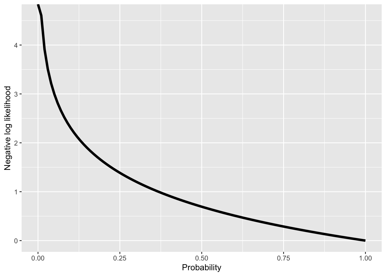
Due to the fact that computers have numerical issues when calculating with very small numbers, i.e. probabilities, we don’t work with probabilities, but instead the natural logarithm of the probabilities (in R this is the log() function).
very_small_number <- 1e-6
very_small_number
[1] 1e-06log(very_small_number)[1] -13.81551A further point is that, by convention, most existing routines for optimizing functions perform minimization, instead of maximization. Therefore, if we want to use functions, such as e.g. optim() in R, we need to minimize the negative log likelihood. This is equivalent to maximizing the likelihood; minimizing the negative log likelihood results in finding the set of parameters for which the probability of the data is maximal.
Generate some data with known parameters
Generate RTs from the diffusion model as data.
It is important to note that the *diffusion() functions take the absolute starting as an argument, instead of the relative starting point. For this reason, we need to compute the absolute starting as \(z = bias * a\). If the relative bias is 0.5, meaning that it is halfway between the boundaries, then the absolute starting point is z = 0.5 * a.
set.seed(54)
rts <- rdiffusion(n = 500,
                  a=genparams["a"],
                  v=genparams["v"],
                  t0=genparams["t0"],
                  z=genparams["z"],
s=0.1) 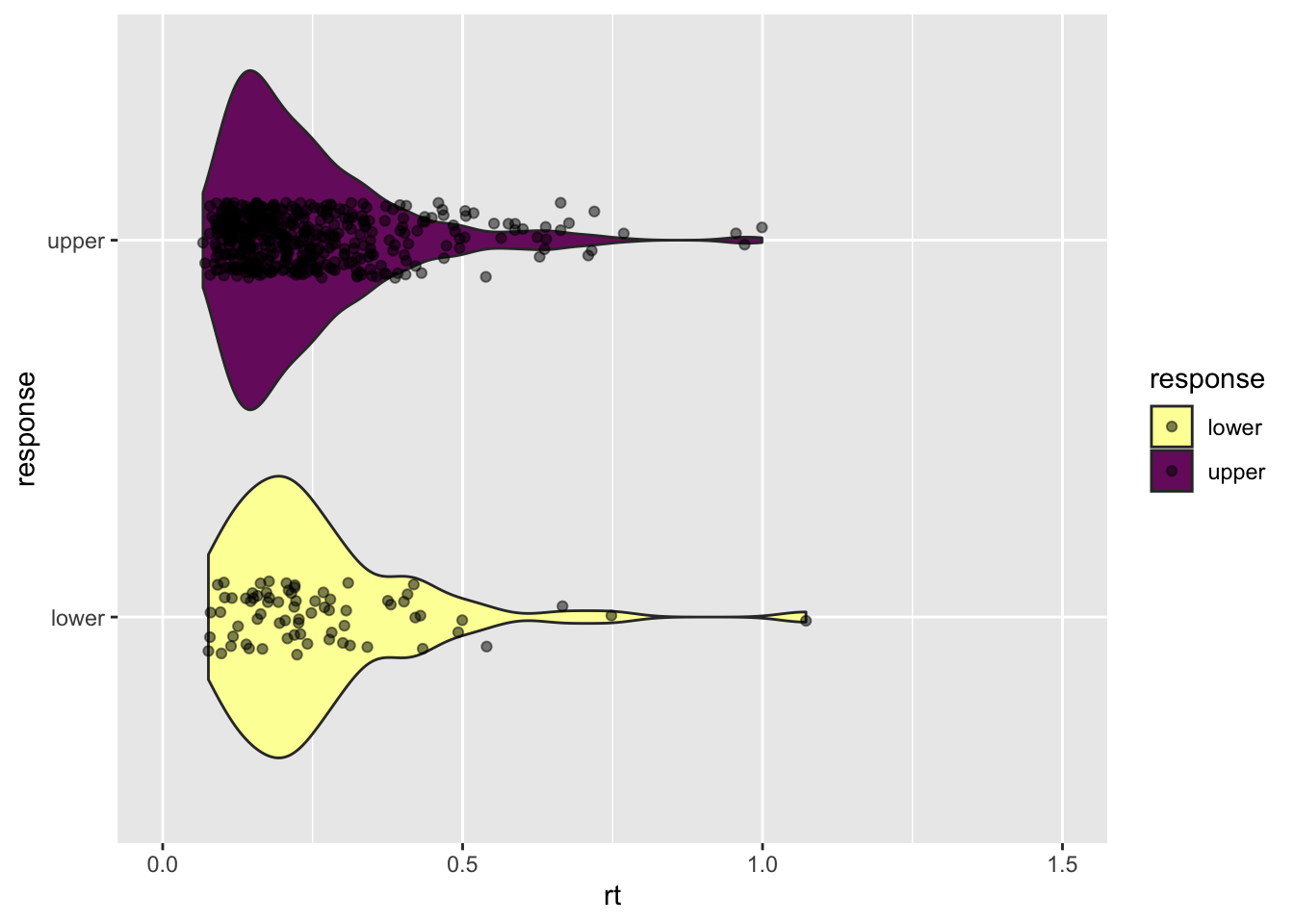
Define log likelihood function
This function returns the negative log probability of the data, given the parameters.
diffusionloglik <- function(pars, rt, response)
{
  likelihoods <- ddiffusion(rt, response=response,
                          a=pars["a"],
                          v=pars["v"],
                          t0=pars["t0"],
                          z=pars["z"],
                          s=0.1)
  return(-sum(log(likelihoods)))
}
Generate starting values for parameters
Estimate parameters
Now, we can evaluate the density function for the DDM, given, the initial parameters:
pars <- init_params

lik <- ddiffusion(rt = rts$rt,
           response = rts$response,
           a = pars["a"],
           v = pars["v"],
           t0 = pars["t0"],
           z = pars["z"],
           s = 0.1)
Next, we can compute the negative log likelihood. If you look at this vector, you will see that there a number of data points for which the log likelihood is -Inf, meaning that the probability of that data point given the initial parameters is \(0\).
This means that we should try to make our function robust; we will do so in the next exercise.
loglik <- log(lik)We can also use our function to calculate the negative log likelihood.
diffusionloglik(init_params, rt = rts$rt,
           response = rts$response)
[1] 503.2724Now, we can repeatedly evaluate the log likelihood, and adjust the parameters so that the negative log likelihood becomes successively smaller. To do this, we use the R function optim().
fit <- optim(init_params,
             diffusionloglik,
             gr = NULL,
             rt = rts$rt,
response = rts$response)fit$par
a v z t0
0.09861885 0.18515304 0.04884865 0.05056087
$value
[1] -200.4542
$counts
function gradient
255 NA
$convergence
[1] 0
$message
NULLCompare estimated parameters to true parameters
round(fit$par, 3) a v z t0
0.099 0.185 0.049 0.051 genparams a v z t0
0.10 0.20 0.05 0.05 Example: full DDM
diffusionloglik <- function(pars, rt, response)
{
  likelihoods <- tryCatch(ddiffusion(rt, response=response,
                          a=pars["a"],
                          v=pars["v"],
                          t0=pars["t0"],
                          z=0.5*pars["a"],
                          sz=pars["sz"],
                          st0=pars["st0"],
                          sv=pars["sv"],s=.1,precision=1),
                        error = function(e) 0)

  if (any(likelihoods==0)) return(1e6)
  return(-sum(log(likelihoods)))
} rts <- rdiffusion(500, a=genparms["a"],
v=genparms["v"],
t0=genparms["t0"],
z=0.5*genparms["a"],
d=0,
sz=genparms["sz"],
sv=genparms["sv"],
st0=genparms["st0"],
s=.1) #now estimate parameters
fit2 <- optim(sparms, diffusionloglik, gr = NULL,
rt=rts$rt, response=rts$response)round(fit2$par, 3) a v t0 sz st0 sv
0.107 0.230 0.500 0.066 0.189 0.073 genparms a v t0 sz st0 sv
0.10 0.20 0.50 0.05 0.20 0.05 Reuse
Citation
@online{ellis2022,
  author = {Andrew Ellis},
  title = {Evidence {Accumulation} {Models:} {II}},
  date = {2022-05-03},
  url = {https://kogpsy.github.io/neuroscicomplabFS22//pages/chapters/10_evidence_accumulation_2.html},
  langid = {en}
}