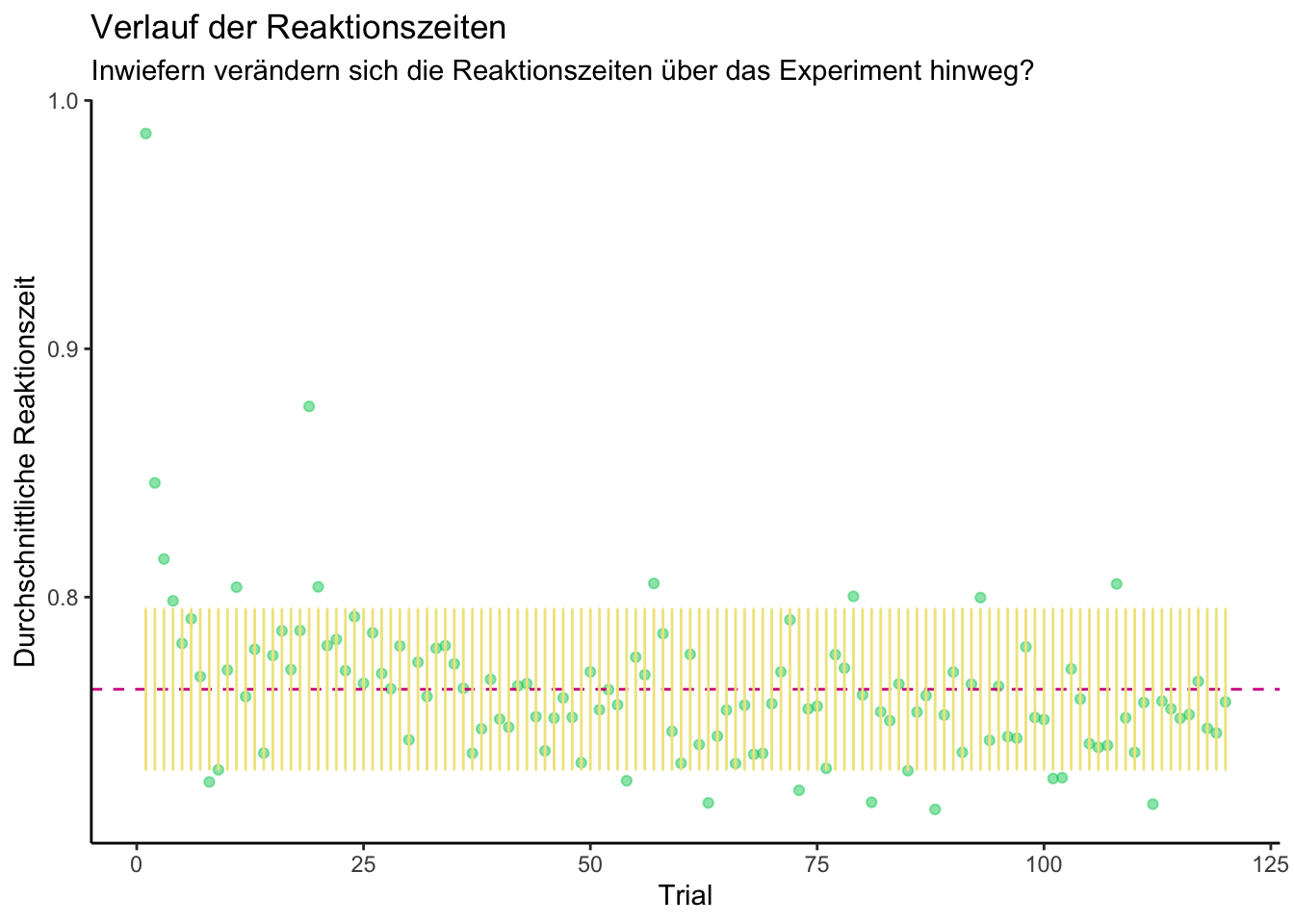
# Inwiefern verändern sich die Reaktionszeiten über das Experiment hinweg?# Numerischen Vektor herstellen:d$rt <-as.numeric(as.character(d$rt))# Gruppieren nach 'id' und Berechnen des Mittelwerts von 'rt' pro Versuchspersonmean_rt_by_trial <- d %>%group_by(trial) %>%summarise(mean_rt =mean(rt, na.rm =TRUE))# Ausgabe der durchschnittlichen Reaktionszeit pro Versuchspersonprint(mean_rt_by_trial)mean_mean_rt <-mean(mean_rt_by_trial$mean_rt)# Ausgabe des Durchschnitts der durchschnittlichen Reaktionszeitenprint(mean_mean_rt)# Standardabweichung berechnen:sd_mean_rt <-sd(mean_rt_by_trial$mean_rt)print(sd_mean_rt)# Plot erstellenggplot(mean_rt_by_trial, aes(x = trial, y = mean_rt, group = trial)) +geom_line(alpha =0.5) +geom_point(alpha =0.5, color ="springgreen3") +geom_hline(yintercept = mean_mean_rt, linetype ="dashed", color ="violetred") +geom_errorbar(yintercept = mean_mean_rt, ymin = mean_mean_rt - sd_mean_rt, ymax = mean_mean_rt + sd_mean_rt, color ="khaki", width =0.1) +labs(x ="Trial", y ="Durchschnittliche Reaktionszeit", subtitle ="Inwiefern verändern sich die Reaktionszeiten über das Experiment hinweg?") +ggtitle("Verlauf der Reaktionszeiten") +theme_classic()
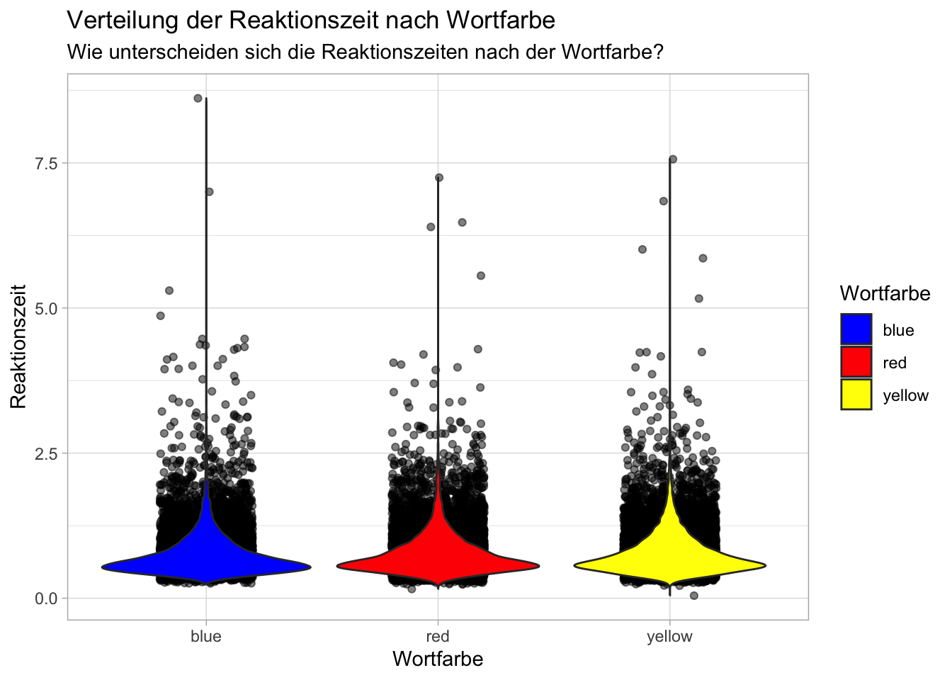
p = d |>ggplot(aes(x = color, y = rt, fill = color)) +geom_jitter(position =position_jitter(width =0.2), color ="black", size =1.5, alpha =0.5) +geom_violin() +scale_fill_manual(values =c("blue", "red", "yellow")) +labs(title ="Verteilung der Reaktionszeit nach Wortfarbe",subtitle ="Wie unterscheiden sich die Reaktionszeiten nach der Wortfarbe?",x ="Wortfarbe",y ="Reaktionszeit",fill ="Wortfarbe" ) +theme_light()p
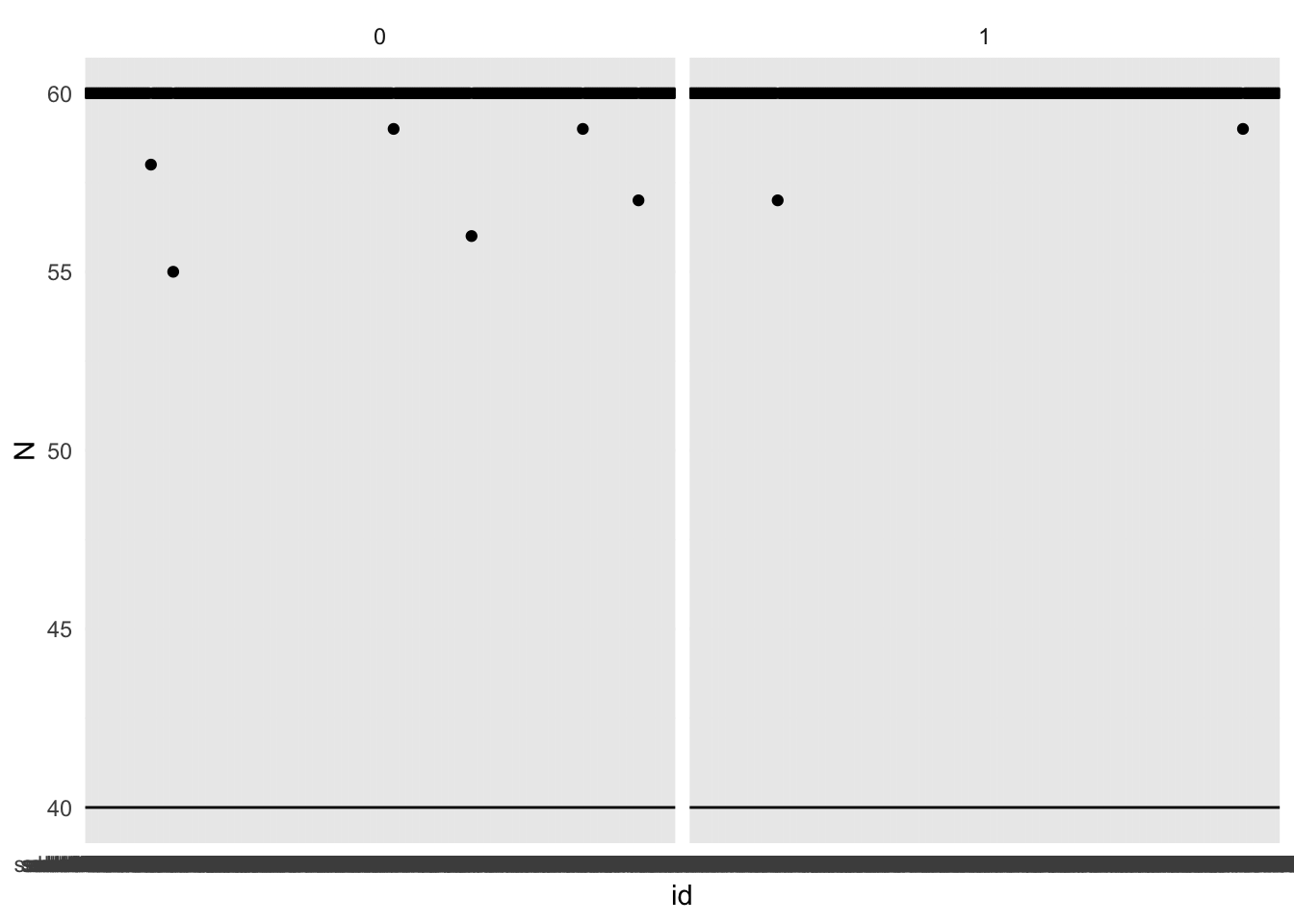
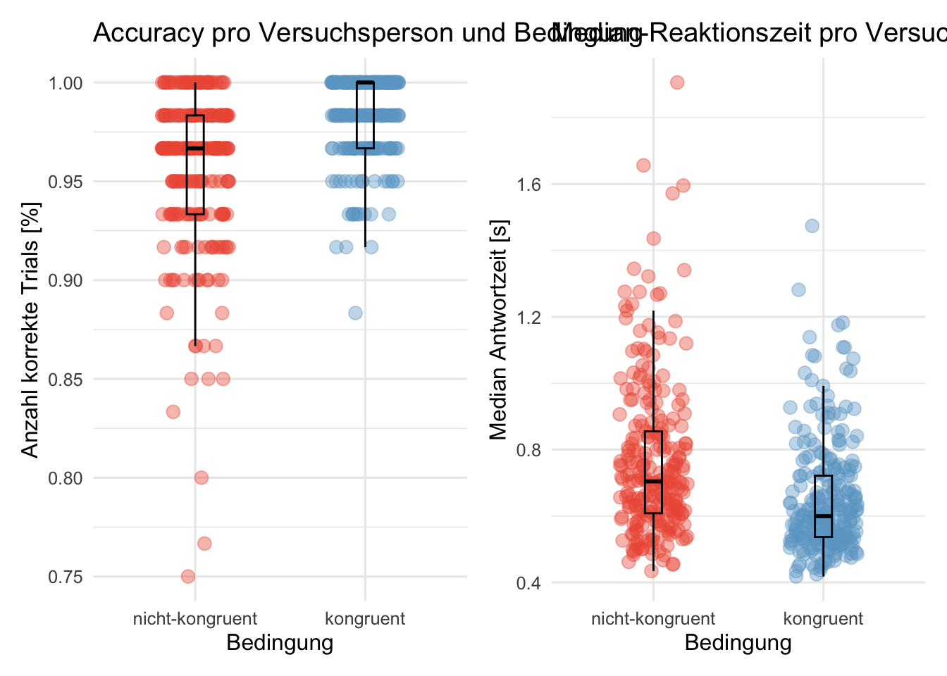
# Beginnen Sie hier mit Ihrem Code:# Ziel: Accuracy pro Person und Condition (congruent/nicht-congruent)# Wir brauchen die Accuracy der Bedingung (congruent/nicht congruent) für alle Vpn.# Dann wollen wir noch ein Mittelmass über Boxplot verwenden# Textvariablen zu Faktoren umwandeln# d %>%# mutate(across(where(is.character), as.factor))# d %>%# slice_head(n= 10)# Gibt es fehlende Werte im Datensatz?# naniar::vis_miss(d)# Ja es gibt fehlende Werte in den Reaktionszeiten# Die fehlenden Werte in den Reaktionszeiten genauer anschauend_missings <- d |> naniar::add_label_missings() |>filter(any_missing =="Missing")# head(d_missings)#Trials, die fehlende Werte in den Reaktionszeiten beinhalten, werden ausgeschlossen:d <- d %>%filter(rt !="NA")# Überprüfen: Hat das ausschliessen geklappt?# naniar::vis_miss(d)# Ja, es gibt keine fehlenden Werte mehr# Auschluss von Reaktionszeiten unter 100ms und unter 10 Sekundend <- d %>%filter(rt >0.09& rt <10)# Daten gruppieren nach ID und Bedingung: Anzahl Trials, Accuracy und mittlere Reaktionszeit berechnenacc_rt_individual <- d %>%group_by(id, congruent) %>%summarise(N =n(),ncorrect =sum(corr),accuracy =mean(corr),median_rt =median(rt) )# Plot: Wie viele Trials pro Bedingung hat jede Versuchsperson gelöst?acc_rt_individual %>%ggplot(aes(x = id, y = N)) +geom_point() +facet_wrap(~ congruent) +geom_hline(yintercept =40) +# Horizontale Linie einfügentheme_minimal()# Datensatz mit allen Ids, welche in mind. einer Condition nicht alle 60 Trials gelöst hattenn_exclusions <- acc_rt_individual %>%filter(N <60)# Wir schliessen alle Vpn aus, die in mind. einer Bedingung nicht alle 60 Trials gelöst hattend <- d %>%filter(!id %in% n_exclusions$id)# Wir gruppieren nochmals nach ID und Bedingung: Anzahl Trials, Accuracy und mittlere Reaktionszeit berechnen.# (Diesmal aber ohne die Subjekte, die nicht in beiden Bedingungen 60 Trials hatten)d_acc_rt_individual <- d %>%group_by(id, congruent) %>%summarise(N =n(),ncorrect =sum(corr),accuracy =mean(corr),median_rt =median(rt) )# Der dazugehörige Plot bestätigt, dass wir alles richtig gemacht haben.d_acc_rt_individual %>%ggplot(aes(x = id, y = N)) +geom_point() +facet_wrap(~ congruent) +geom_hline(yintercept =40) +# Horizontale Linie einfügentheme_minimal()# Für weitere Analysen verwenden wir nun d_acc_rt_individual####################################### Wir schauen nun, ob es betreffend Accuracy noch Ausreisser im Datensatz gibt.# Als Ausreisser definieren wir eine Person, die weniger als 40% Accuracy hatte# Trials nach accuracy einteilen. Dazu fügen wir dem Datensatz d_acc_rt_individual eine neue Variable "performance" hinzud_acc_rt_individual <- d_acc_rt_individual %>%mutate(performance =case_when( accuracy >0.75~"good", accuracy <0.4~"bad",TRUE~"chance level") %>%factor(levels =c("good", "chance level", "bad")))# Outlier visualisieren# d_acc_rt_individual %>%# ggplot(aes(x = id, y = accuracy, color = performance, shape = performance)) +# geom_point(size = 2, alpha = 0.6) +# geom_point(data = filter(d_acc_rt_individual, performance != "OK"),# alpha = 0.9) +# facet_grid(~congruent) +# scale_color_manual(values = c("gray40", "steelblue", "red")) +# geom_hline(yintercept = 0.5, linetype='dotted', col = 'black')+# annotate("text", x = "sub-36817827", y = 0.5, label = "chance level", vjust = -1, size = 3) +# theme_minimal(base_size = 12)# Wir sehen im Plot direkt, dass es einen Ausreisser gibt.# Es handelt sich um folgendes Subjekt:accuracy_outliers <- d_acc_rt_individual %>%filter(performance =="bad")# Wir schliessen den Ausreisser aus dem Datensatz aus:d_acc_rt_individual <- d_acc_rt_individual %>%filter(performance !="bad")# Nun kommen wir endlich zum Herzstück. Wir plotten wir die accuracy für jede Person und Bedingung# Plot p1: Accuracy pro Vpn und Bedingung# (Wichtig: Wir müssen ggplot sagen, dass "congruent" eine kategoriale Variable mit Ausprägungen 0 und 1 ist)p1 <- d_acc_rt_individual |>ggplot(aes(x =factor(congruent, labels =c("nicht-kongruent", "kongruent")), y = accuracy, color =factor(congruent))) +geom_jitter(size =3, alpha =0.4,width =0.2, height =0) +geom_boxplot(width =0.1, alpha =0, color ="black") +scale_color_manual(values =c("0"="tomato2","1"="skyblue3")) +labs(x ="Bedingung",y ="Anzahl korrekte Trials [%]",title ="Accuracy pro Versuchsperson und Bedingung") +theme_minimal(base_size =12) +theme(legend.position ="none")# p1##### Hier ist die eigentliche Aufgabe verwendet. Als Lösung bitte p1 verwenden ########## Zum Spass plotten wir noch Plot p2: Reaktionszeit pro Vpn pro Bedingungp2 <- d_acc_rt_individual |>ggplot(aes(x =factor(congruent, labels =c("nicht-kongruent", "kongruent")), y = median_rt, color =factor(congruent))) +geom_jitter(size =3, alpha =0.4,width =0.2, height =0) +geom_boxplot(width =0.1, alpha =0, color ="black") +scale_color_manual(values =c("0"="tomato2","1"="skyblue3")) +labs(x ="Bedingung",y ="Median Antwortzeit [s]",title ="Median-Reaktionszeit pro Versuchsperson und Bedingung") +theme_minimal(base_size =12) +theme(legend.position ="none")# p2#mittels Patchwork können wir p1 und p2 nebeneinander anzeigen lassen# Patchwork ladenlibrary(patchwork)p1 + p2
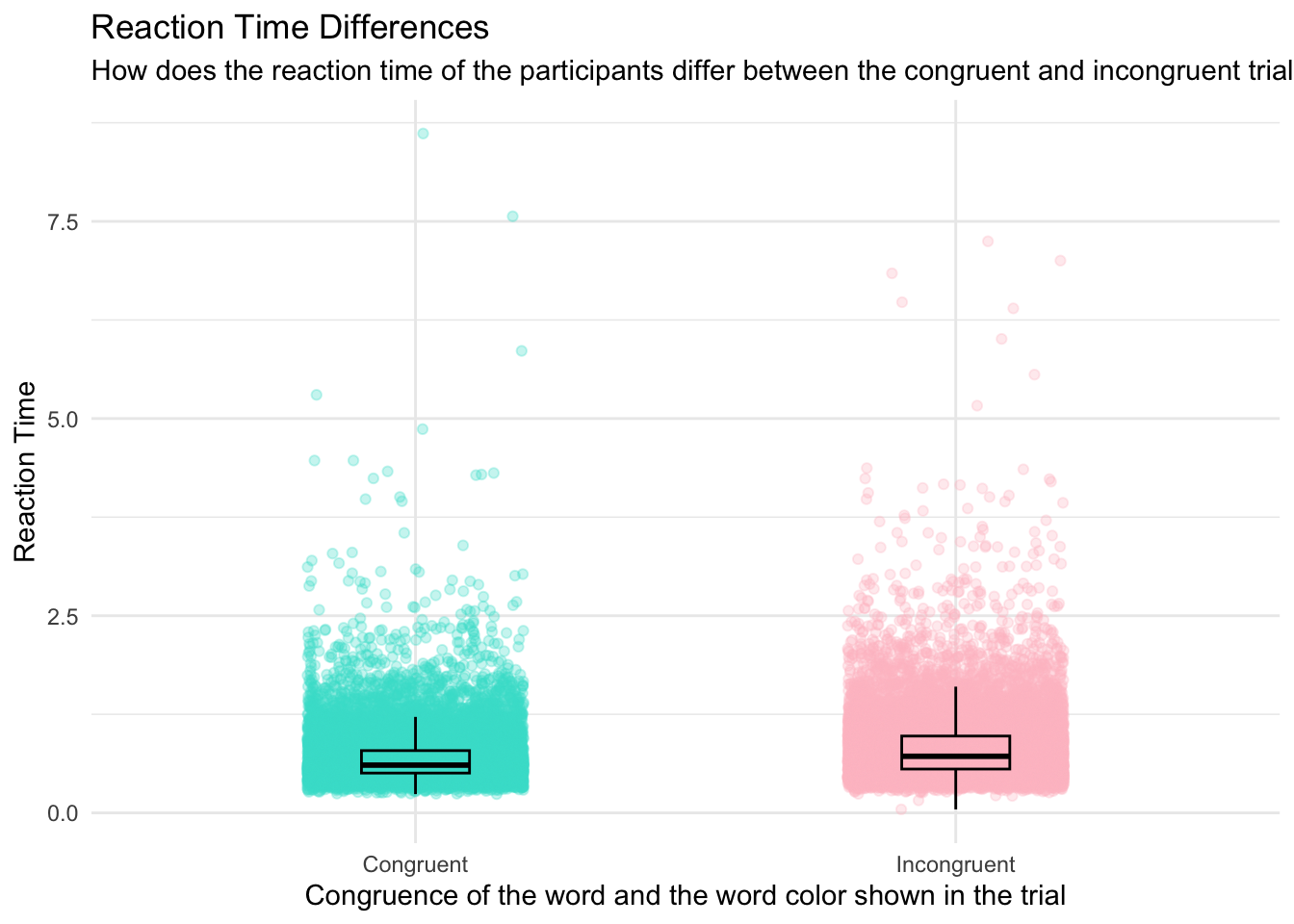
# Beginnen Sie hier mit Ihrem Code:d$Congruence_Label <-ifelse(d$congruent ==0, "Incongruent", "Congruent")p = d |>ggplot(data = d,mapping =aes(x = Congruence_Label, y = rt, color = Congruence_Label)) +geom_jitter(size =1.5, alpha =0.3,width =0.2, height =0) +geom_boxplot(width =0.2, alpha =0, color ="black") +labs(x ="Congruence of the word and the word color shown in the trial",y ="Reaction Time",title ="Reaction Time Differences",subtitle ="How does the reaction time of the participants differ between the congruent and incongruent trials?") +scale_color_manual(values =c("turquoise", "pink"))+theme_minimal() +theme(legend.position ="none")p
# Beginnen Sie hier mit Ihrem Code:# naniar::vis_miss(d)#NA sind weniger als 0.1% in dem ganzen Datsatz und sind alle in der Variable rt -> in Plot werden diese rausgefiltertd<-d %>%mutate(condition=as.factor(congruent))levels(d$condition) <-c("incongruent","congruent")# glimpse(d)#in der Zeilen 13-16 habe ich eine neue Variable kreiiert ("condition"), die ein Vektor der (numerischen) Variable "congruent" istp1=d %>%filter(!is.na(rt)) %>%ggplot(aes(x = condition, y = rt, color = condition))+geom_jitter(size =2, alpha =0.3,width =0.4, height =0.5) +geom_boxplot(width=0.5, alpha=0, color ='black') +scale_y_continuous(limits =c(0, 10))+scale_color_manual(values =c(incongruent ="lightgreen",congruent ="darkgreen"))+labs(x ="Stroop Condition",y ="Reaction Time [s]",title ="Reaction Time (RT)",subtitle ="Is there a difference in RT between conditions?") +theme_minimal(base_size =12) +theme(legend.position ="none")p1
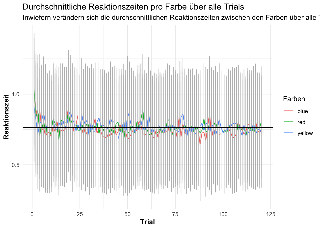
# Inwiefern verändern sich die durchschnittlichen Reaktionszeiten zwischen# den Farben über alle Trials?library(ggplot2)d$rt <-as.numeric(as.character(d$rt))overall_avg_rt <-mean(d$rt)d$rt <-as.numeric(as.character(d$rt))overall_avg_rt <-mean(d$rt, na.rm =TRUE)overall_sd_rt <-sd(d$rt, na.rm =TRUE)# Plot Erstellenp <- d %>%group_by(trial, color) %>%summarise(avg_rt =mean(rt)) %>%ggplot(aes(x = trial, y = avg_rt, color = color)) +geom_line() +geom_errorbar(aes(ymin = avg_rt - overall_sd_rt, ymax = avg_rt + overall_sd_rt),linetype ="solid", color ="grey", width =0.1 ) +labs(x ="Trial",y ="Reaktionszeit",color ="Farben",title ="Durchschnittliche Reaktionszeiten pro Farbe über alle Trials",subtitle ="Inwiefern verändern sich die durchschnittlichen Reaktionszeiten zwischen den Farben über alle Trials? " ) +geom_hline(yintercept = overall_avg_rt, linetype ="solid" , color ="black", linewidth =1) +theme_minimal() +ggtitle("Durchschnittliche Reaktionszeiten pro Farbe über alle Trials") +theme(axis.title.x =element_text(face ="bold"),axis.title.y =element_text(face ="bold") )print(p)
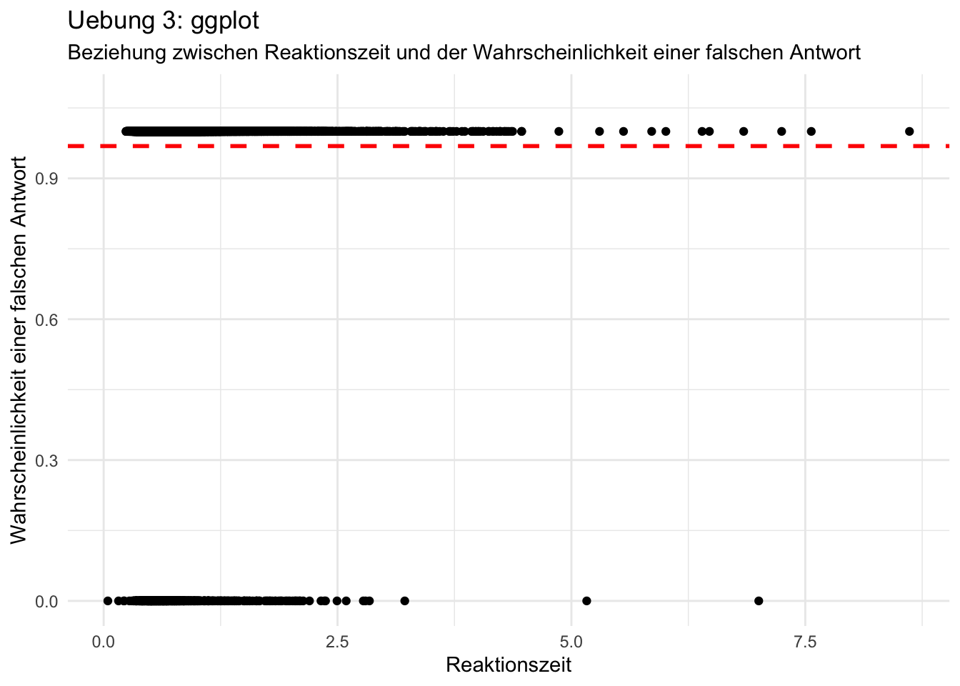
# Beginnen Sie hier mit Ihrem Code:mean_rt <-mean(d$rt)sd_rt <-sd(d$rt)p = d |>ggplot(data = d,mapping =aes(x = rt,y = corr)) +geom_point() +geom_hline(yintercept =mean(d$corr), linetype ="dashed", color ="red", size =1) +# Horizontale Linie für den Mittelwert der Wahrscheinlichkeit falscher Antwortenannotate("text", x = mean_rt, y =mean(d$corr) +0.05, label =paste("Mean RT:", round(mean_rt, 2)), color ="blue", hjust =0) +# Text für den Mittelwert der Reaktionszeitannotate("text", x = mean_rt, y =mean(d$corr) +0.1, label =paste("SD RT:", round(sd_rt, 2)), color ="green", hjust =0) +# Text für die Standardabweichung der Reaktionszeitlabs(title ="Uebung 3: ggplot",subtitle ="Beziehung zwischen Reaktionszeit und der Wahrscheinlichkeit einer falschen Antwort",x ="Reaktionszeit", y ="Wahrscheinlichkeit einer falschen Antwort") +theme_minimal()p
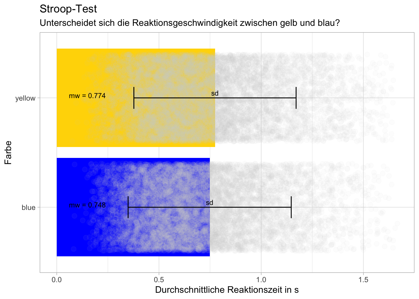
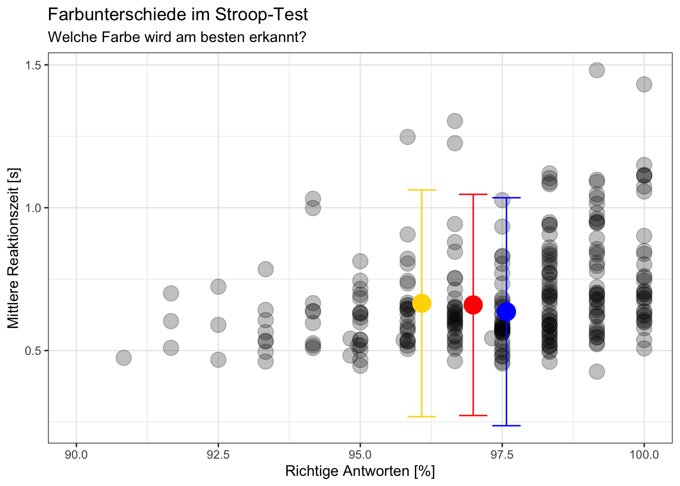
#Beginnen Sie hier mit Ihrem Codelibrary(ggplot2)library(dplyr)# Daten zusammenfassen und fehlende Werte entfernend_summary <- d %>%filter(!is.na(rt)) %>%group_by(color) %>%summarise(mean_rt =mean(rt),sd_rt =sd(rt)) # Standardabweichung berechnen# Rohdaten verarbeiten damit nur relevanter Bereich gezeigt wirdd <- d %>%filter(rt <1.5)# Erstellen einer Zuordnung von Farben zu Farbencolor_mapping <-c("blue"="blue", "yellow"="gold")# ggplot mit individuellen Farben für jeden Balken, Standardabweichung und Rohdatenp <-ggplot(d_summary %>%filter(color %in%c("yellow", "blue")), aes(y = color, x = mean_rt, fill = color)) +geom_bar(stat ='identity') +geom_point(data = d %>%filter(color %in%c("yellow", "blue")), aes(x = rt, group = color), position =position_jitter(width =0.2), color ="lightgrey", size =2.5, alpha =0.05)+geom_errorbar(data = d_summary %>%filter(color %in%c("yellow", "blue")), aes(xmin = mean_rt - sd_rt, xmax = mean_rt + sd_rt), width =0.2)+# Fehlerbalken für Standardabweichunggeom_text(aes(label =paste("mw =", round(mean_rt, 3)), x =0.15), vjust =0, color ="black", size =3, data = d_summary %>%filter(color %in%c("yellow", "blue"))) +# Mittelwert als Zahl in die Balken schreibengeom_text(aes(label =paste("sd")), vjust =-0.5, color ="black", size =3, data = d_summary %>%filter(color %in%c("yellow", "blue")))+# sd beschriftenscale_fill_manual(values = color_mapping) +labs(title ="Stroop-Test",subtitle ="Unterscheidet sich die Reaktionsgeschwindigkeit zwischen gelb und blau?",y ="Farbe",x ="Durchschnittliche Reaktionszeit in s") +theme_light() +theme(legend.position ="none") # Farbskala entfernenp
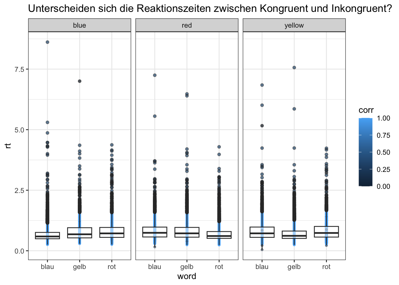
#Plot erstellenlibrary(ggplot2)d %>%ggplot(aes(word,rt,colour = corr))+geom_point(size =1, alpha =0.5)+facet_wrap(~color)+geom_boxplot(alpha =0.5)+theme_bw()+labs(title ="Unterscheiden sich die Reaktionszeiten zwischen Kongruent und Inkongruent?")
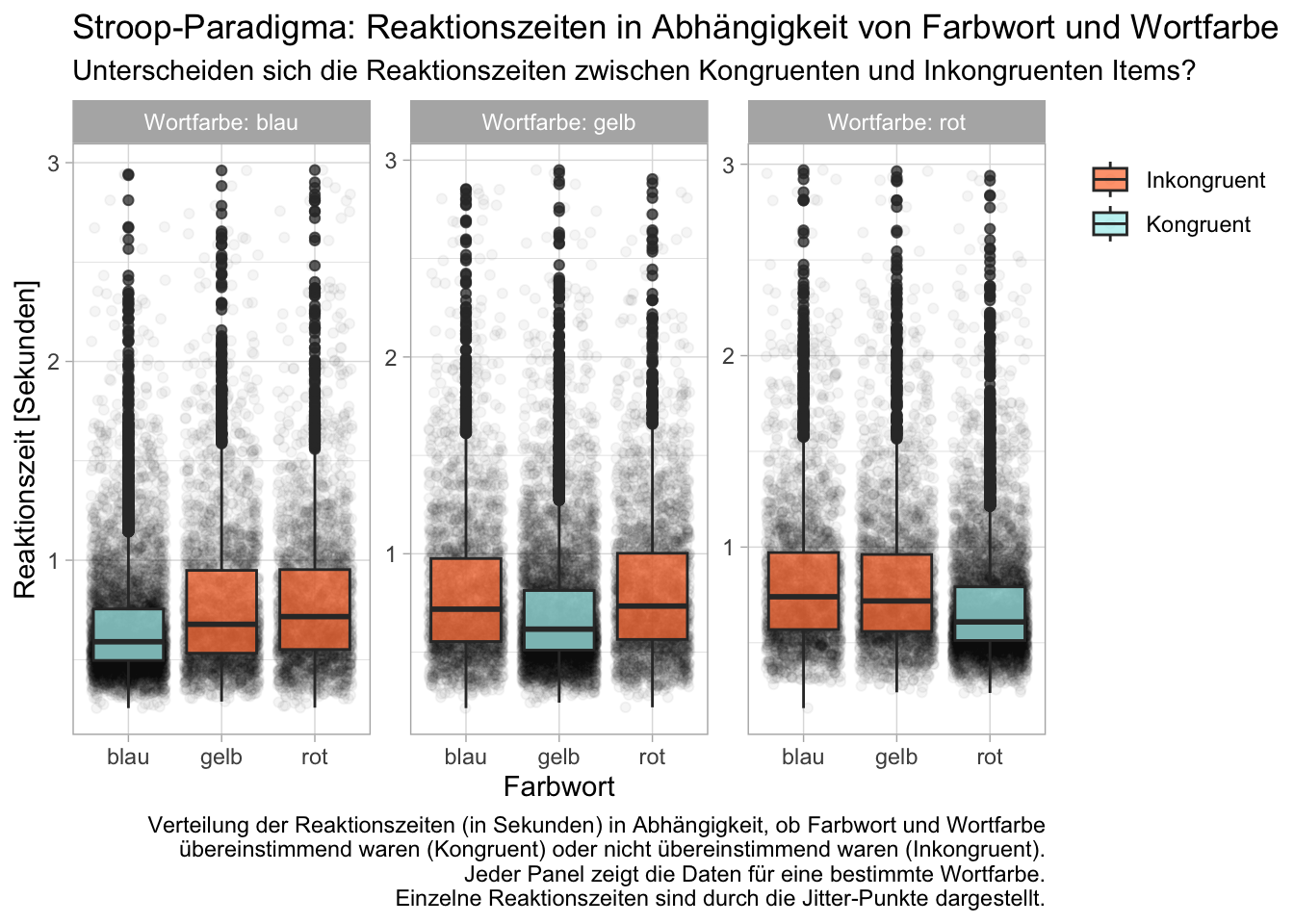
library(ggplot2)library(dplyr)# Alle mit Reaktionszeit grösser als 3.00 Sekunden und kleiner als 0.09 entfernend <- d %>%filter(rt >0.09& rt <=3.00)# Erstellen eines neuen Datenrahmens mit den Titeln für die Facetsfacet_labels <-data.frame(color =unique(d$color), facet_title =c("Wortfarbe: rot", "Wortfarbe: gelb", "Wortfarbe: blau"))# Verbindung von Facet-Titeln mit dem Datensatzd_with_labels <-left_join(d, facet_labels, by ="color")# Erstellen des Plots mit individuellen Facet-Titelnplot <-ggplot(data = d_with_labels, aes(x = word,y = rt,fill =factor(congruent))) +geom_jitter(alpha = .04) +#Boxplot soll über dem jitter seingeom_boxplot(alpha = .75) +# Achsenbeschriftungenlabs(title ="Stroop-Paradigma: Reaktionszeiten in Abhängigkeit von Farbwort und Wortfarbe",subtitle ="Unterscheiden sich die Reaktionszeiten zwischen Kongruenten und Inkongruenten Items?",x ="Farbwort",y ="Reaktionszeit [Sekunden]",fill ="Kongruenz",caption ="Verteilung der Reaktionszeiten (in Sekunden) in Abhängigkeit, ob Farbwort und Wortfarbe übereinstimmend waren (Kongruent) oder nicht übereinstimmend waren (Inkongruent). Jeder Panel zeigt die Daten für eine bestimmte Wortfarbe. Einzelne Reaktionszeiten sind durch die Jitter-Punkte dargestellt.") +scale_fill_manual(values =c("0"="sienna1", "1"="paleturquoise2"),labels =c("0"="Inkongruent", "1"="Kongruent")) +theme_light() +theme(legend.title =element_blank()) +#Kein Titel für die Legendetheme(legend.justification ="top") +# Legende obenrechts platzierenfacet_wrap(~facet_title, scales ="free")plot
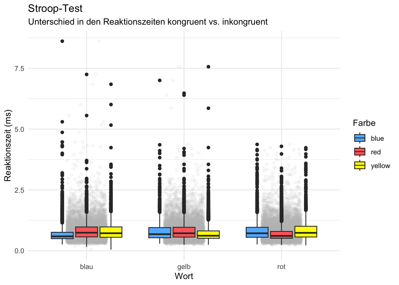
# Beginnen Sie hier mit Ihrem Code:library(ggplot2)p = d %>%ggplot(aes(x = word, y = rt, fill = color)) +geom_jitter(color="grey", position =position_jitter(width =0.2), alpha =0.1) +labs(title ="Stroop-Test",subtitle ="Unterschied in den Reaktionszeiten kongruent vs. inkongruent",x ="Wort",y ="Reaktionszeit (ms)",fill ="Farbe" ) +geom_boxplot() +theme_minimal() +scale_fill_manual(values =c("steelblue1", "indianred1", "yellow"))print(p)
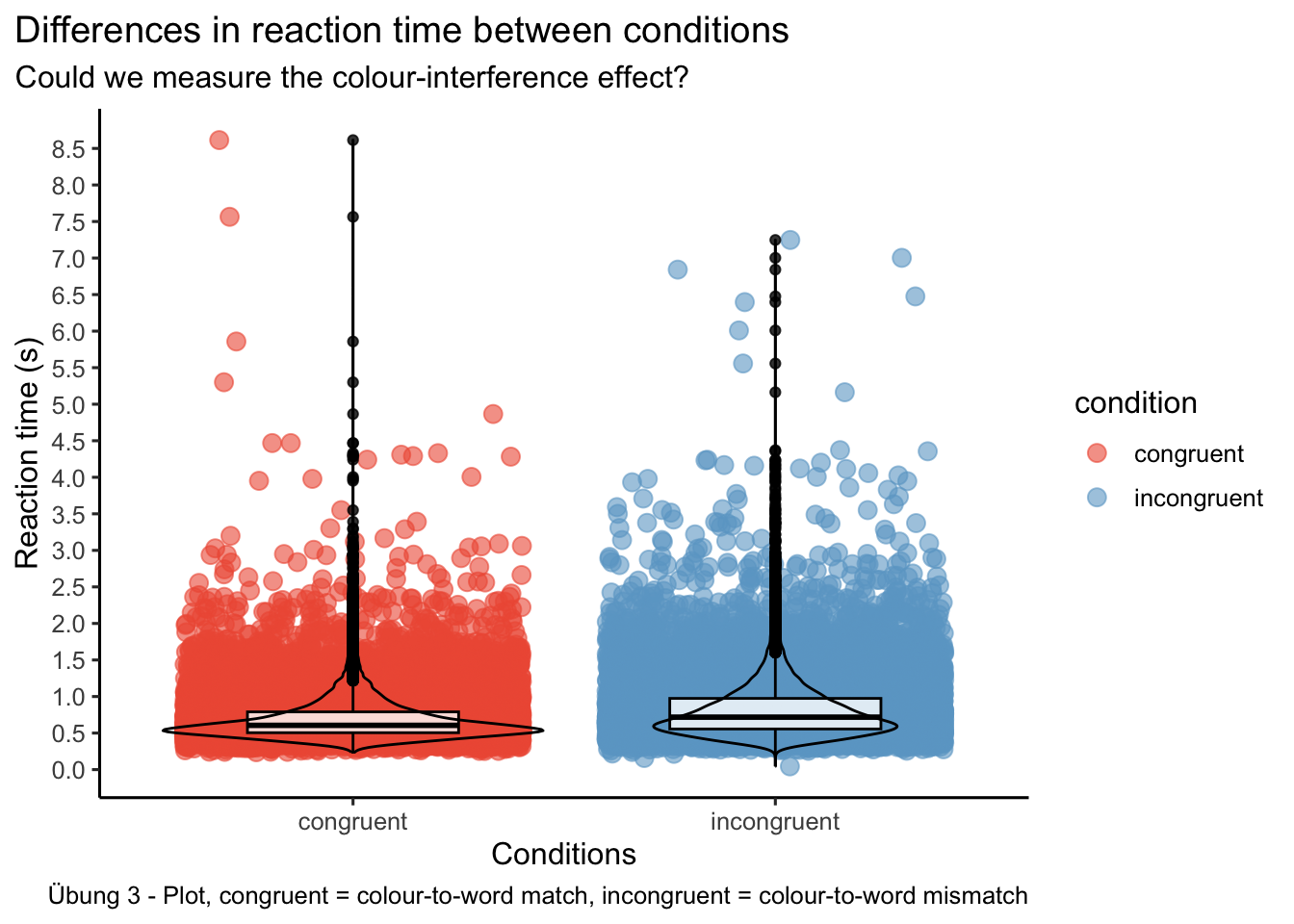
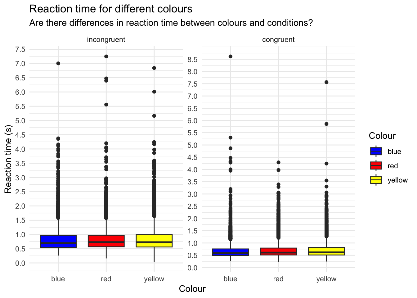
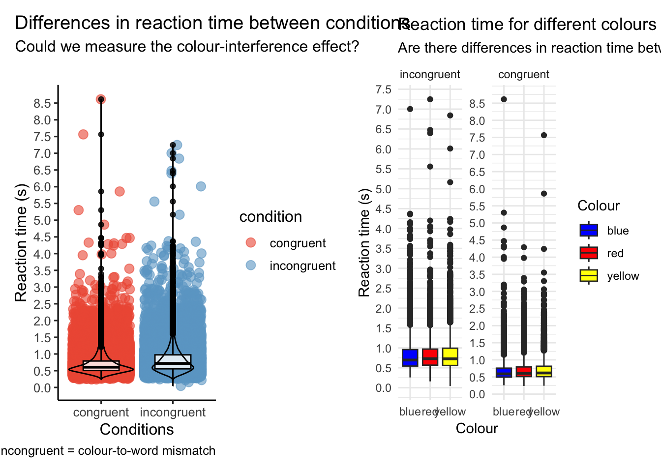
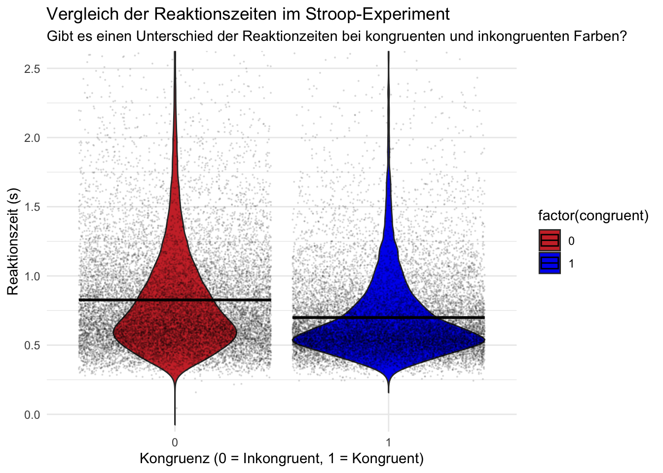
# Beginnen Sie hier mit Ihrem Code:library(tidyverse)library(patchwork)# Daten laden# d <- read.csv("data/dataset_stroop_clean.csv")# d %>% slice_head(n = 10)# Diagnostik#view(d)# naniar::vis_miss(d)# summary(d$rt)# eigentlich sollte im Zuge des Data Wranglings alle NA's entfernt worden sein (daher _clean) aber mit summary(d$rt) erscheinen 19 NA's# NA's entfernend_missings <- d |> naniar::add_label_missings() |>filter(any_missing =="Missing")# head(d_missings)# Variable congruent in conditions mit congruent/incongruent umwandelnd_conditions <- d %>%na.omit() %>%mutate(condition =case_when(congruent ==1~"congruent", congruent ==0~"incongruent"))# Plot 1: Reaktionszeitsunterschiede zwischen conditionsp1 <- d_conditions %>%ggplot(aes(x = condition, y = rt, color = condition)) +geom_jitter(size =3, alpha =0.6,width =0.4, height =0) +geom_boxplot(width =0.5, alpha =0.8, color ="black") +geom_violin(alpha =0, color ="black") +scale_color_manual(values =c(congruent ="tomato2",incongruent ="skyblue3"))+labs(title ="Differences in reaction time between conditions",subtitle ="Could we measure the colour-interference effect?",caption ="Übung 3 - Plot, congruent = colour-to-word match, incongruent = colour-to-word mismatch",x ="Conditions",y ="Reaction time (s)") +theme_classic(base_size =12) +theme(legend.position ="right",plot.title.position ="plot")+scale_y_continuous(breaks =seq(0, max(d_conditions$rt), by =0.5))p1# Für versch. Farben und conditionsd_farben <- d_conditions %>%filter(color %in%c("yellow", "red", "blue"))d_farben$congruent <-factor(d_farben$congruent)# Plot erstellend_farben$congruent <-factor(d_farben$congruent, levels =c(0, 1), labels =c("incongruent", "congruent"))p2 <-ggplot(d_farben, aes(x = color, y = rt, fill = color)) +geom_boxplot(position =position_dodge(width =0.8)) +labs(title ="Reaction time for different colours",subtitle ="Are there differences in reaction time between colours and conditions?",x ="Colour",y ="Reaction time (s)",fill ="Colour") +facet_wrap(~ congruent, scales ="free") +scale_fill_manual(values =c("blue"="blue", "yellow"="yellow", "red"="red")) +theme_minimal() +theme(legend.position ="right") +scale_y_continuous(breaks =seq(0, max(d_conditions$rt), by =0.5))p2# zusammenfügenp1 + p2
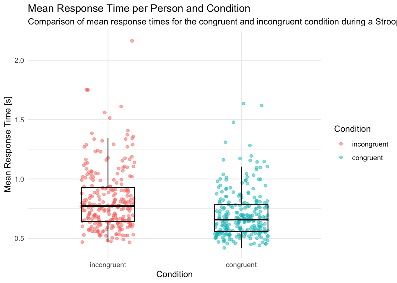
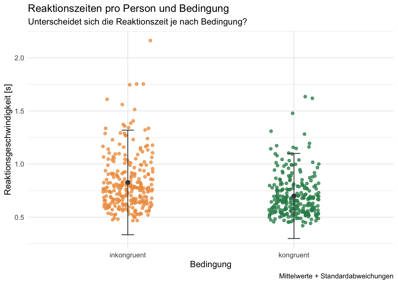
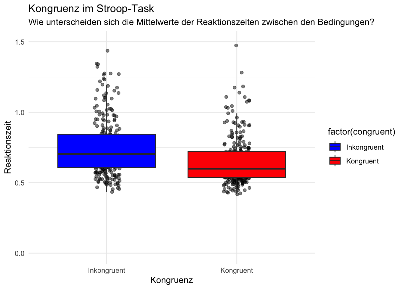
# Beginnen Sie hier mit Ihrem Code:p <- d|>mutate(congruent =as.factor(congruent))|>mutate(congruent =fct_recode(congruent ,incongruent ="0" ,congruent ="1")) |>filter(rt !="NA")|>group_by(id, congruent) |>summarise(N =n(), mean_rt =mean(rt))|>ggplot(aes(x = congruent, y = mean_rt, color = congruent)) +geom_jitter(size =1.5, alpha =0.5,width =0.2, height =0) +geom_boxplot(width =0.4, alpha =0, color ="black") +labs(x ="Condition",y ="Mean Response Time [s]",title ="Mean Response Time per Person and Condition",subtitle ="Comparison of mean response times for the congruent and incongruent condition during a Stroop test",fill ="Condition",colour ="Condition" ) +theme_minimal()p
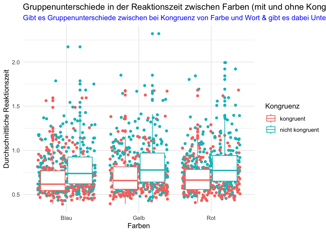
# Beginnen Sie hier mit Ihrem Code:d_filtered = d |>filter(!is.na(rt))group_color = d_filtered |>group_by(id, color, congruent) |>summarise(mean_rt =mean(rt))group_color <- group_color %>%mutate(congruent =recode(congruent, `0`="nicht kongruent", `1`="kongruent"))group_color <- group_color %>%mutate(color =recode(color, `yellow`="Gelb", `red`="Rot", `blue`="Blau"))visual <- group_color %>%ggplot(aes(x = color, y = mean_rt, color = congruent)) +geom_jitter() +geom_boxplot()+labs(title ="Gruppenunterschiede in der Reaktionszeit zwischen Farben (mit und ohne Kongruenz zwischen Farbe & Wort)",subtitle ="Gibt es Gruppenunterschiede zwischen bei Kongruenz von Farbe und Wort & gibt es dabei Unterschiede zwischen den Farben?",x ="Farben", y="Durchschnittliche Reaktionszeit", color ="Kongruenz")+theme_minimal() +theme(plot.subtitle =element_text(color ="blue"))visual
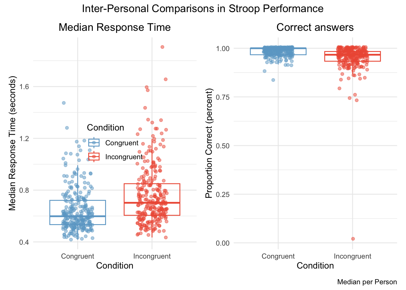
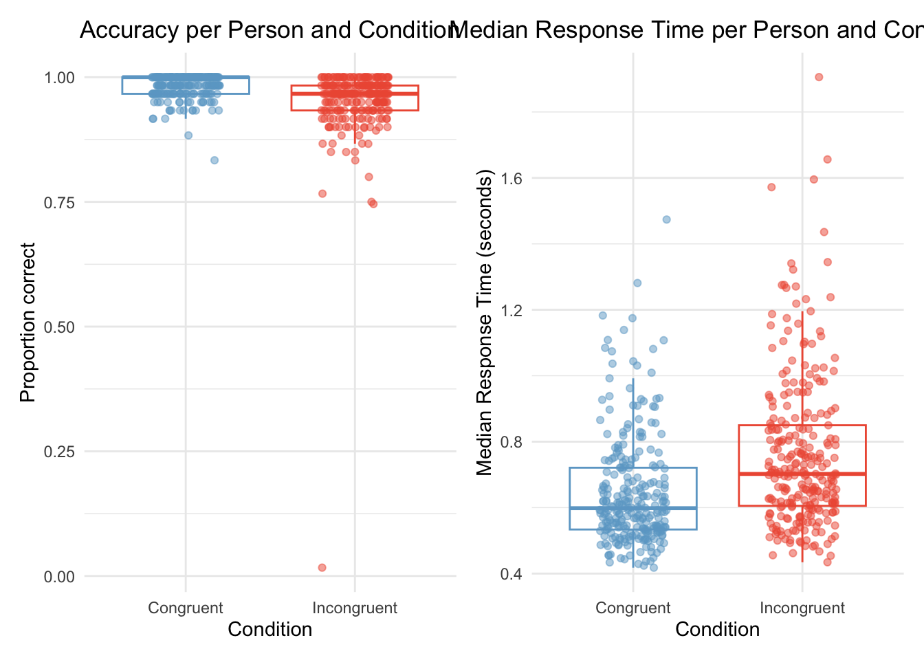
# Beginnen Sie hier mit Ihrem Code:p = d |>mutate(across(where(is.character), as.factor))# Datensatz anschauen# d |># slice_head(n = 10)#Die Frage mit der ich mich befasse, ist, wie sich die Accuracy und die Response Time#zwischen den Bedinungen (Congruent vs. Incongruent) unterscheidet.#Dazu erstelle ich eine Grafik, die den Unterschied in der Accuracy bzw. der Response Time#der einzelnen Personen zwischen den beiden Bedingungen vergleicht.# library(naniar)# naniar::vis_miss(d)d_missings <- d |> naniar::add_label_missings() |>filter(any_missing =="Missing")# head(d_missings)# zu schnelle und zu langsame Antworten ausschliessend <- d |>filter(rt >0.09& rt <15)# Daten gruppieren: Anzahl Trials, Accuracy und mittlere Reaktionszeit berechnenacc_rt_individual <- d |>group_by(id, congruent) |>summarise(N =n(),ncorrect =sum(corr),accuracy =mean(corr),median_rt =median(rt)) |>ungroup() %>%mutate(Condition =ifelse(congruent ==1, "Congruent", "Incongruent"))# Plot: Anzahl TrconditionCall()# Plot: Anzahl Trials pro Bedingung für jede Versuchsperson# acc_rt_individual |># ggplot(aes(x = id, y = N)) +# geom_point() +# facet_wrap(~ congruent) +# geom_hline(yintercept = 40) + # Horizontale Linie einfügen# theme_minimal()# Datensatz mit allen Ids, welche zuwenig Trials hattenn_exclusions <- acc_rt_individual |>filter(N <40)# Aus dem Hauptdatensatz diese Ids ausschliessend <- d |>filter(!id %in% n_exclusions$id)# Checkd_acc_rt_individual <- d |>group_by(id, congruent) |>summarise(N =n(),ncorrect =sum(corr),accuracy =mean(corr),median_rt =median(rt)) |>ungroup() %>%mutate(Condition =ifelse(congruent ==1, "Congruent", "Incongruent"))# Plot accuracy per person and conditionp1 <- d_acc_rt_individual |>ggplot(aes(x = Condition, y = accuracy, color = Condition)) +geom_point(position =position_jitter(width =0.2), alpha =0.5) +scale_color_manual(values =c(Incongruent ="tomato2",Congruent ="skyblue3")) +geom_boxplot(alpha =0, outlier.shape =NA) +labs(title ='Accuracy per Person and Condition',x ='Condition',y ='Proportion correct') +theme_minimal() +theme(plot.title =element_text(hjust =0.5)) +theme(legend.position ='none')p2 <- d_acc_rt_individual |>ggplot(aes(x = Condition, y = median_rt, color = Condition)) +geom_point(position =position_jitter(width =0.2), alpha =0.5) +scale_color_manual(values =c(Incongruent ="tomato2",Congruent ="skyblue3")) +geom_boxplot(alpha =0, outlier.shape =NA) +labs(title ='Median Response Time per Person and Condition',x ='Condition',y ='Median Response Time (seconds)') +theme_minimal() +theme(plot.title =element_text(hjust =0.5)) +theme(legend.position ="none")p1 + p2#Die Antwort auf meine Fragestellung:#Die Accuracy ist in der Congruenten Bedingung etwas höher als in der Incongruenten Bedinung.#Die Response Time ist in der Congruenten Bedinung schneller als in der Incongruenten Bedingung.#Dies entspricht meinen Erwartungen
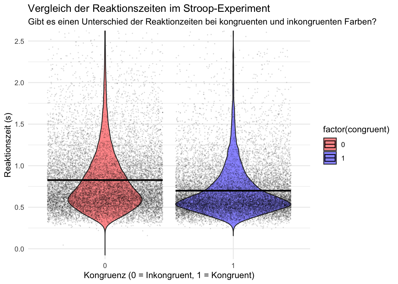
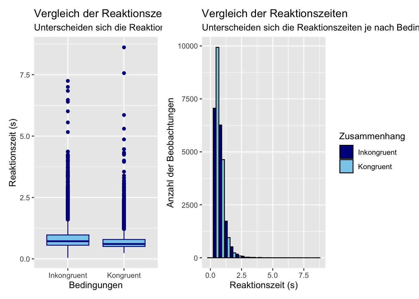
# Beginnen Sie hier mit Ihrem Code:#Version 1: Boxplotp1 = d %>%mutate(Zusammenhang =if_else(congruent ==1, "Kongruent", "Inkongruent")) %>%ggplot((aes(x=Zusammenhang, y=rt))) +geom_boxplot(fill ="skyblue", color ="darkblue") +labs(title ="Vergleich der Reaktionszeiten",subtitle ="Unterscheiden sich die Reaktionszeiten je nach Bedingung?",x ="Bedingungen",y ="Reaktionszeit (s)")#Version 2: Histogrammp2 = d %>%mutate(Zusammenhang =if_else(congruent ==1, "Kongruent", "Inkongruent")) %>%ggplot(aes(x = rt, fill = Zusammenhang)) +geom_histogram(position ="dodge", bins =20, color ="black") +labs(title ="Vergleich der Reaktionszeiten",subtitle ="Unterscheiden sich die Reaktionszeiten je nach Bedingung?",x ="Reaktionszeit (s)",y ="Anzahl der Beobachtungen") +scale_fill_manual(values =c("Kongruent"="skyblue", "Inkongruent"="darkblue"))library(patchwork)p1+p2
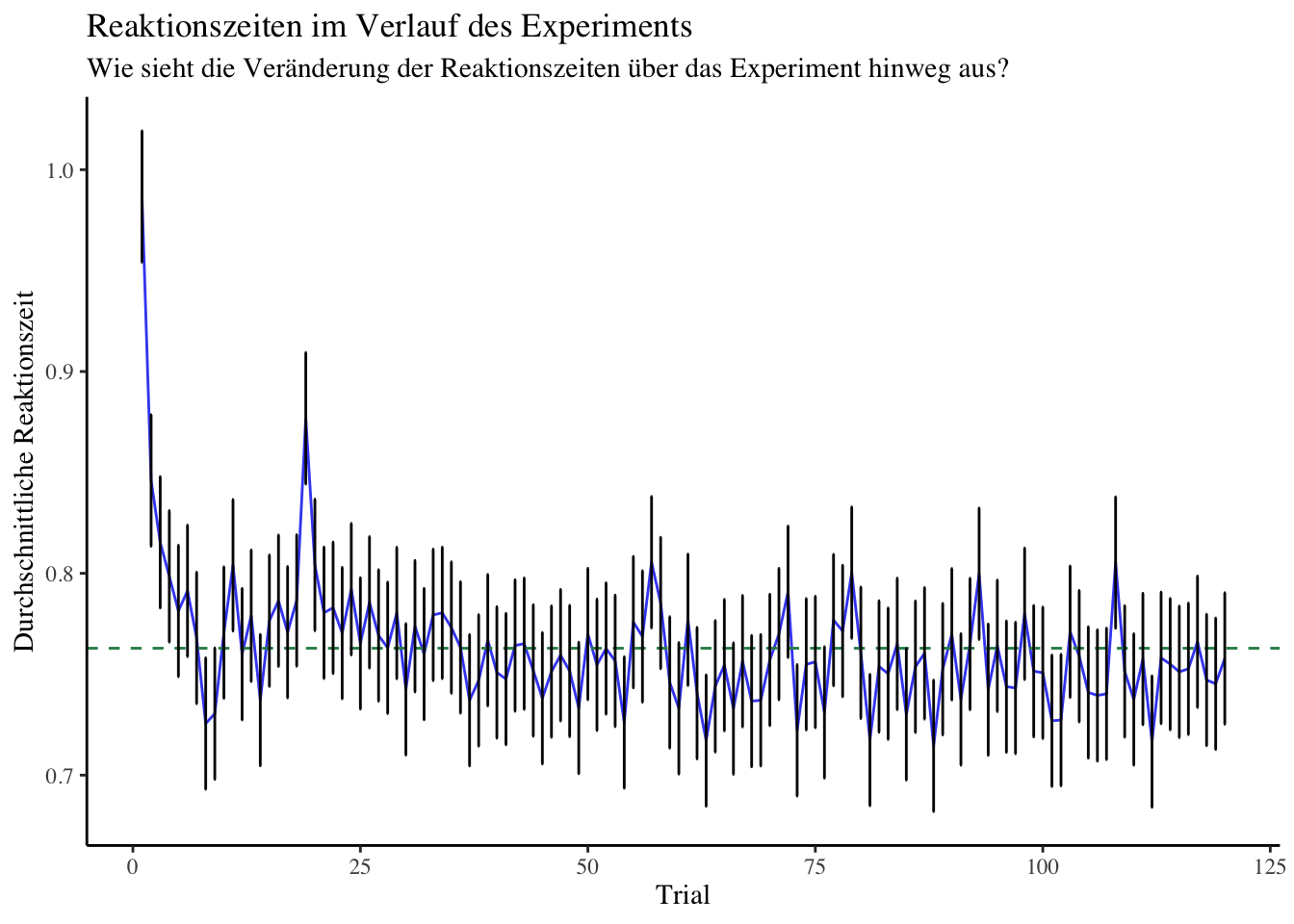
# Frage: wie sieht die Veränderung der Reaktionszeiten über das Experiment# hinweg aus?# Beginnen Sie hier mit Ihrem Code:#numerischer Vektor erstellend$rt <-as.numeric(as.character(d$rt))#Gruppieren nach "id" und Berechnen des Mittelwerts von "rt" pro Versuchspersonmean_rt_by_trial <- d %>%group_by(trial) %>%summarise(mean_rt =mean(rt, na.rm =TRUE))#Ausgabe der durchschnittlichen Reaktionszeit pro Versuchsperson# print(mean_rt_by_trial)#Berechnung des Durchschnitts der durchschnittlichen Reaktionszeitenmean_mean_rt <-mean(mean_rt_by_trial$mean_rt)#Berechnung der Standardabweichungmean_sd_rt <-sd(mean_rt_by_trial$mean_rt)#Plot erstellenggplot(mean_rt_by_trial, aes(x = trial, y = mean_rt)) +geom_line(alpha =0.8, color ="blue2") +geom_hline(yintercept = mean_mean_rt, linetype ="dashed", color ="seagreen4") +geom_errorbar(aes(ymin = mean_rt - mean_sd_rt, ymax = mean_rt + mean_sd_rt), width =0.2, color ="grey1") +labs(x ="Trial", y ="Durchschnittliche Reaktionszeit", subtitle ="Wie sieht die Veränderung der Reaktionszeiten über das Experiment hinweg aus?") +ggtitle("Reaktionszeiten im Verlauf des Experiments") +theme_classic() +theme(text =element_text(family ="Times"))