Daten importieren: Teil 2

Mehrere Datensätze programmatisch bearbeiten.

Author

Affiliation

Andrew Ellis

Kognitive Psychologie, Wahrnehmung und Methodenlehre, Universität Bern

Published

March 20, 2023

Lernziele

In der heutigen Sitzung lernen wir:

Arbeitsschritte automatisieren: mehrere Datensätze automatisch importieren
Mit ChatGPT Code verstehen

Datacamp

Falls Sie eine Einführung in Programmierkonzepte (Conditionals and Control Flow, Functions, Loops) benötigen, empfehlen wir Ihnen den Datacamp Kurs Intermediate R.

Mehrere Datensätze bearbeiten

library(tidyverse)

── Attaching core tidyverse packages ──────────────────────── tidyverse 2.0.0 ──
✔ dplyr     1.1.1     ✔ readr     2.1.4
✔ forcats   1.0.0     ✔ stringr   1.5.0
✔ ggplot2   3.4.2     ✔ tibble    3.2.1
✔ lubridate 1.9.2     ✔ tidyr     1.3.0
✔ purrr     1.0.1     
── Conflicts ────────────────────────────────────────── tidyverse_conflicts() ──
✖ dplyr::filter() masks stats::filter()
✖ dplyr::lag()    masks stats::lag()
ℹ Use the conflicted package (<http://conflicted.r-lib.org/>) to force all conflicts to become errors

Meist werden Daten für jede Versuchsperson einzeln abgespeichert. Um nicht jeden Datensatz einzeln einlesen zu müssen können wir Schleifen (loops) und Funktionen nutzen. Schleifen und Funktionen sind immer extrem zeitsparend, wenn ein Prozess wiederholt werden muss. Dies kommt in der Verarbeitung grosser Datensätze häufig vor. Zudem werden so Tippfehler vermieden, die häufig passieren, wenn man dreissig Mal dasselbe schreiben muss.

Nun werden wir dasselbe wie im Teil 1 machen; dort haben wir ein csv File importiert, und dessen Variablen ausgewählt und umbenannt. Dieses Mal wollen wir aber alle .csv Files laden, die in einem Ordner gespeichert sind.

In Ihrem Rstudio Projekt sind die Files im Ordner data gespeichert.

Alle Files in einem Ordner auflisten

Zuerst erstellen wir mit list.files() eine Liste aller .csv Files im Ordner data.

datadir <- "data"

csv_files <- datadir |>
    list.files(pattern = "csv", full.names = TRUE)

csv_files

[1] "data/JH_rdk-discrimination_2022_Mar_07_1403.csv"   
[2] "data/NS_rdk-discrimination_2022_Mar_07_1331.csv"   
[3] "data/rh_rdk-discrimination_2022_Mar_02_1105.csv"   
[4] "data/sb_rdk-discrimination_2022_Mar_06_0746.csv"   
[5] "data/SS91_rdk-discrimination_2022_Mar_06_0953.csv" 
[6] "data/VP1_rdk-discrimination_2022_Mar_07_1237.csv"  
[7] "data/VP2_rdk-discrimination_2022_Mar_07_1302.csv"  
[8] "data/VPN01_rdk-discrimination_2022_Mar_01_2142.csv"
[9] "data/VPN02_rdk-discrimination_2022_Mar_01_2208.csv"

csv_files enthält nun die “Pfade” zu allen .csv Files im Ordner data. Diese Pfade können nun einzeln and read_csv() übergeben werden.

Mit `for`-Loop

Zuerst brauchen wir eine Liste, in die wir die Daten einlesen können. Wir erstellen eine Liste mit der Länge der Anzahl Files, die wir haben.

data_list <- vector("list", length(csv_files))

Nun können wir entweder über die Elemente der Liste iterieren, oder über die Indizes. Wir wählen letzteres, da wir die Indizes später für die Zuweisung der Daten verwenden können.

for (i in seq_along(csv_files)) {
            df <- read_csv(csv_files[i])
            data_list[[i]] <- df
}

Das Resultat ist eine Liste, in deren Elementen die neun csv Files gepesichert sind.

length(data_list)

[1] 9

Diese wollen wir nun zu einem Dataframe zusammenfügen. Dazu können wir do.call() verwenden. do.call() nimmt eine Funktion und eine Liste als Argumente. Die Liste werden wiederum als Argumente der Funktion verwendet.

data_loop <- do.call(rbind, data_list)

head(data_loop)

# A tibble: 6 × 40
  cue   direction practice_block_loop.thisRepN practice_block_loop.thisTrialN
  <chr> <chr>                            <dbl>                          <dbl>
1 none  right                                0                              0
2 left  right                                0                              1
3 right right                                0                              2
4 left  left                                 0                              3
5 none  left                                 0                              4
6 right left                                 0                              5
# ℹ 36 more variables: practice_block_loop.thisN <dbl>,
#   practice_block_loop.thisIndex <dbl>, main_blocks_loop.thisRepN <dbl>,
#   main_blocks_loop.thisTrialN <dbl>, main_blocks_loop.thisN <dbl>,
#   main_blocks_loop.thisIndex <dbl>, static_isi.started <dbl>,
#   static_isi.stopped <dbl>, fixation_pre.started <dbl>,
#   fixation_pre.stopped <chr>, image.started <dbl>, image.stopped <chr>,
#   fixation_post.started <dbl>, fixation_post.stopped <chr>, …

Mit `map` und `list_rbind`

Dasselbe können wir auch mit map() machen. Da auch hier der Output eine Liste ist, müssen wir diese auch zu einem Dataframe zusammenfügen. Dazu können wir list_rbind() verwenden.

data <- csv_files |> 
    map(read_csv) |>
    list_rbind()

data |>
  slice_head(n = 20)

# A tibble: 20 × 40
   cue   direction practice_block_loop.thisRepN practice_block_loop.thisTrialN
   <chr> <chr>                            <dbl>                          <dbl>
 1 none  right                                0                              0
 2 left  right                                0                              1
 3 right right                                0                              2
 4 left  left                                 0                              3
 5 none  left                                 0                              4
 6 right left                                 0                              5
 7 <NA>  <NA>                                NA                             NA
 8 right right                               NA                             NA
 9 right right                               NA                             NA
10 none  right                               NA                             NA
11 none  right                               NA                             NA
12 left  left                                NA                             NA
13 none  right                               NA                             NA
14 none  left                                NA                             NA
15 left  left                                NA                             NA
16 left  right                               NA                             NA
17 none  right                               NA                             NA
18 none  left                                NA                             NA
19 left  left                                NA                             NA
20 left  left                                NA                             NA
# ℹ 36 more variables: practice_block_loop.thisN <dbl>,
#   practice_block_loop.thisIndex <dbl>, main_blocks_loop.thisRepN <dbl>,
#   main_blocks_loop.thisTrialN <dbl>, main_blocks_loop.thisN <dbl>,
#   main_blocks_loop.thisIndex <dbl>, static_isi.started <dbl>,
#   static_isi.stopped <dbl>, fixation_pre.started <dbl>,
#   fixation_pre.stopped <chr>, image.started <dbl>, image.stopped <chr>,
#   fixation_post.started <dbl>, fixation_post.stopped <chr>, …

Nun können wir wie in Teil 1 die Practice Trials entfernen.

data  <- data |>  
        filter(!is.na(main_blocks_loop.thisN)) |>
        select(-contains("practice_block_loop"))

Variablen auswählen und umbennen

Wir eliminieren die Variablen, die wir nicht brauchen (ISI, Fixationskreuz, Zeitangaben der Bilder, etc.).

data <- data |>
    select(-contains("static"),
           -contains("fixation"),
           -contains("image"),
           -contains("instruction"),
           -contains("feedback"))

Zum Schluss geben wir den Variablen, die wir behalten, noch deskriptivere Namen.

data <- data |>
    select(trial = main_blocks_loop.thisN,
           ID = Pseudonym,
           cue,
           direction,
           response = dots_keyboard_response.keys,
           rt = dots_keyboard_response.rt)

data |>
  slice_head(n = 20)

# A tibble: 20 × 6
   trial ID    cue   direction response    rt
   <dbl> <chr> <chr> <chr>     <chr>    <dbl>
 1     0 JH    right right     j        0.714
 2     1 JH    right right     j        0.627
 3     2 JH    none  right     f        0.670
 4     3 JH    none  right     j        0.574
 5     4 JH    left  left      j        0.841
 6     5 JH    none  right     j        0.668
 7     6 JH    none  left      j        1.12 
 8     7 JH    left  left      f        0.640
 9     8 JH    left  right     f        1.13 
10     9 JH    none  right     j        1.03 
11    10 JH    none  left      f        1.35 
12    11 JH    left  left      f        0.688
13    12 JH    left  left      f        0.721
14    13 JH    none  left      f        0.655
15    14 JH    right right     j        1.02 
16    15 JH    none  right     j        1.12 
17    16 JH    left  left      f        1.08 
18    17 JH    right left      f        0.643
19    18 JH    right right     j        0.716
20    19 JH    left  left      f        0.578

Neue Variablen definieren

Eine Antwort ist korrekt, wenn die gewählte Richtung der Richtung des Dot-Stimulus entspricht. Zuvor definieren wir zwei Variablen: choice besteht aus den Angaben “right” und “left”, response ist eine numerische Version davon (0 = “left”, 1 = “right”).

Korrekte Antworten

data <- data |>
    mutate(choice = if_else(response == "j", "right", "left"),
           response = if_else(choice == "right", 1, 0))

correct ist TRUE wenn choice == direction, FALSE wenn nicht. Wir konvertieren diese logische Variable mit as.numeric() in eine numerische Variable. as.numeric() konvertiert TRUE in 1 und FALSE in 0.

Lösung

as.numeric(c(TRUE, FALSE))

[1] 1 0

data <- data |>
    mutate(correct = as.numeric(choice == direction))

glimpse(data)

Rows: 1,440
Columns: 8
$ trial     <dbl> 0, 1, 2, 3, 4, 5, 6, 7, 8, 9, 10, 11, 12, 13, 14, 15, 16, 17…
$ ID        <chr> "JH", "JH", "JH", "JH", "JH", "JH", "JH", "JH", "JH", "JH", …
$ cue       <chr> "right", "right", "none", "none", "left", "none", "none", "l…
$ direction <chr> "right", "right", "right", "right", "left", "right", "left",…
$ response  <dbl> 1, 1, 0, 1, 1, 1, 1, 0, 0, 1, 0, 0, 0, 0, 1, 1, 0, 0, 1, 0, …
$ rt        <dbl> 0.7136441, 0.6271285, 0.6703410, 0.5738488, 0.8405913, 0.667…
$ choice    <chr> "right", "right", "left", "right", "right", "right", "right"…
$ correct   <dbl> 1, 1, 0, 1, 0, 1, 0, 1, 0, 1, 1, 1, 1, 1, 1, 1, 1, 1, 1, 1, …

Wir schauen uns die ersten 20 Zeilen an.

data |> 
  slice_head(n = 20)

# A tibble: 20 × 8
   trial ID    cue   direction response    rt choice correct
   <dbl> <chr> <chr> <chr>        <dbl> <dbl> <chr>    <dbl>
 1     0 JH    right right            1 0.714 right        1
 2     1 JH    right right            1 0.627 right        1
 3     2 JH    none  right            0 0.670 left         0
 4     3 JH    none  right            1 0.574 right        1
 5     4 JH    left  left             1 0.841 right        0
 6     5 JH    none  right            1 0.668 right        1
 7     6 JH    none  left             1 1.12  right        0
 8     7 JH    left  left             0 0.640 left         1
 9     8 JH    left  right            0 1.13  left         0
10     9 JH    none  right            1 1.03  right        1
11    10 JH    none  left             0 1.35  left         1
12    11 JH    left  left             0 0.688 left         1
13    12 JH    left  left             0 0.721 left         1
14    13 JH    none  left             0 0.655 left         1
15    14 JH    right right            1 1.02  right        1
16    15 JH    none  right            1 1.12  right        1
17    16 JH    left  left             0 1.08  left         1
18    17 JH    right left             0 0.643 left         1
19    18 JH    right right            1 0.716 right        1
20    19 JH    left  left             0 0.578 left         1

Cue-Bedingungsvariable

Nun brauchen wir eine Variable, die angibt, ob die Bedingung “neutral”, “valid” oder “invalid” ist. Wir erstellen eine neue Variable condition und füllen sie mit case_when() mit den Werten “neutral”, “valid” oder “invalid”. case_when() erlaubt, mehrere if_else()-Bedingungen zu kombinieren. So wird hier der Variablen condition der Wert neutral zugewiesen, wenn cue == "none" ist. Falls cue == direction ist, wird der Wert valid zugewiesen. Falls cue != direction ist, wird der Wert invalid zugewiesen.

data <- data |>
    mutate(condition = case_when(cue == "none" ~ "neutral",
                                 cue == direction ~ "valid",
                                 cue != direction ~ "invalid"))

data |> 
  slice_head(n = 20)

# A tibble: 20 × 9
   trial ID    cue   direction response    rt choice correct condition
   <dbl> <chr> <chr> <chr>        <dbl> <dbl> <chr>    <dbl> <chr>    
 1     0 JH    right right            1 0.714 right        1 valid    
 2     1 JH    right right            1 0.627 right        1 valid    
 3     2 JH    none  right            0 0.670 left         0 neutral  
 4     3 JH    none  right            1 0.574 right        1 neutral  
 5     4 JH    left  left             1 0.841 right        0 valid    
 6     5 JH    none  right            1 0.668 right        1 neutral  
 7     6 JH    none  left             1 1.12  right        0 neutral  
 8     7 JH    left  left             0 0.640 left         1 valid    
 9     8 JH    left  right            0 1.13  left         0 invalid  
10     9 JH    none  right            1 1.03  right        1 neutral  
11    10 JH    none  left             0 1.35  left         1 neutral  
12    11 JH    left  left             0 0.688 left         1 valid    
13    12 JH    left  left             0 0.721 left         1 valid    
14    13 JH    none  left             0 0.655 left         1 neutral  
15    14 JH    right right            1 1.02  right        1 valid    
16    15 JH    none  right            1 1.12  right        1 neutral  
17    16 JH    left  left             0 1.08  left         1 valid    
18    17 JH    right left             0 0.643 left         1 invalid  
19    18 JH    right right            1 0.716 right        1 valid    
20    19 JH    left  left             0 0.578 left         1 valid

Daten als CSV speichern

An dieser Stelle speichern wir den neu kreierten Datensatz als .csv File in einen Ordner names data_clean. Somit können wir zu einem späteren Zeitpunkt die Daten einfach importieren, ohne die ganzen Schritte wiederholen zu müssen.

data |> write_csv(file = "data_clean/rdkdata.csv")

Gruppierungsvariablen

Alle Gruppierungsvariablen sollten nun zu Faktoren konvertiert werden.

data <- data |>
    mutate(across(where(is.character), as_factor))

glimpse(data)

Rows: 1,440
Columns: 9
$ trial     <dbl> 0, 1, 2, 3, 4, 5, 6, 7, 8, 9, 10, 11, 12, 13, 14, 15, 16, 17…
$ ID        <fct> JH, JH, JH, JH, JH, JH, JH, JH, JH, JH, JH, JH, JH, JH, JH, …
$ cue       <fct> right, right, none, none, left, none, none, left, left, none…
$ direction <fct> right, right, right, right, left, right, left, left, right, …
$ response  <dbl> 1, 1, 0, 1, 1, 1, 1, 0, 0, 1, 0, 0, 0, 0, 1, 1, 0, 0, 1, 0, …
$ rt        <dbl> 0.7136441, 0.6271285, 0.6703410, 0.5738488, 0.8405913, 0.667…
$ choice    <fct> right, right, left, right, right, right, right, left, left, …
$ correct   <dbl> 1, 1, 0, 1, 0, 1, 0, 1, 0, 1, 1, 1, 1, 1, 1, 1, 1, 1, 1, 1, …
$ condition <fct> valid, valid, neutral, neutral, valid, neutral, neutral, val…

Daten überprüfen

Wir überprüfen, ob die Daten korrekt sind. Dazu schauen wir uns die Anzahl der Trials pro Person und pro Bedingung an. Sie können mehr Zeilen anzeigen, indem sie n = in der Funktion slice_head() ändern.

data |> 
  group_by(ID, condition) |>
  summarise(n_trials = n()) |>
  slice_head(n = 20)

`summarise()` has grouped output by 'ID'. You can override using the `.groups`
argument.

# A tibble: 27 × 3
# Groups:   ID [9]
   ID    condition n_trials
   <fct> <fct>        <int>
 1 JH    valid           64
 2 JH    neutral         80
 3 JH    invalid         16
 4 NS    valid           64
 5 NS    neutral         80
 6 NS    invalid         16
 7 rh    valid           64
 8 rh    neutral         80
 9 rh    invalid         16
10 sb    valid           64
# ℹ 17 more rows

Accuracy pro Person/Bedingung

Nun berechnen wir pro Person und pro Bedingung die Anzahl der korrekten Antworten und die Accuracy. Die Accuracy ist die Anzahl der korrekten Antworten geteilt durch die Anzahl der Trials.

accuracy <- data |>
    group_by(ID, condition) |>
    summarise(N = n(),
              ncorrect = sum(correct),
              accuracy = mean(correct))

`summarise()` has grouped output by 'ID'. You can override using the `.groups`
argument.

accuracy

# A tibble: 27 × 5
# Groups:   ID [9]
   ID    condition     N ncorrect accuracy
   <fct> <fct>     <int>    <dbl>    <dbl>
 1 JH    valid        64       60    0.938
 2 JH    neutral      80       66    0.825
 3 JH    invalid      16       13    0.812
 4 NS    valid        64       58    0.906
 5 NS    neutral      80       56    0.7  
 6 NS    invalid      16       11    0.688
 7 rh    valid        64       61    0.953
 8 rh    neutral      80       64    0.8  
 9 rh    invalid      16        2    0.125
10 sb    valid        64       62    0.969
# ℹ 17 more rows

Visualisieren

accuracy |> 
  ggplot(aes(x = condition, y = accuracy, fill = condition)) +
  geom_col() +
  geom_line(aes(group = ID), linewidth = 2) +
  geom_point(size = 4) +
  scale_fill_manual(values = c(invalid = "#9E0142",
                    neutral = "#C4C4B7",
                    valid = "#2EC762")) +
  labs(x = "Cue",
      y = "Proportion correct",
      title = "Accuracy per person/condition") +
  facet_wrap(~ID) +
  theme_linedraw(base_size = 28) +
  theme(legend.position = "none")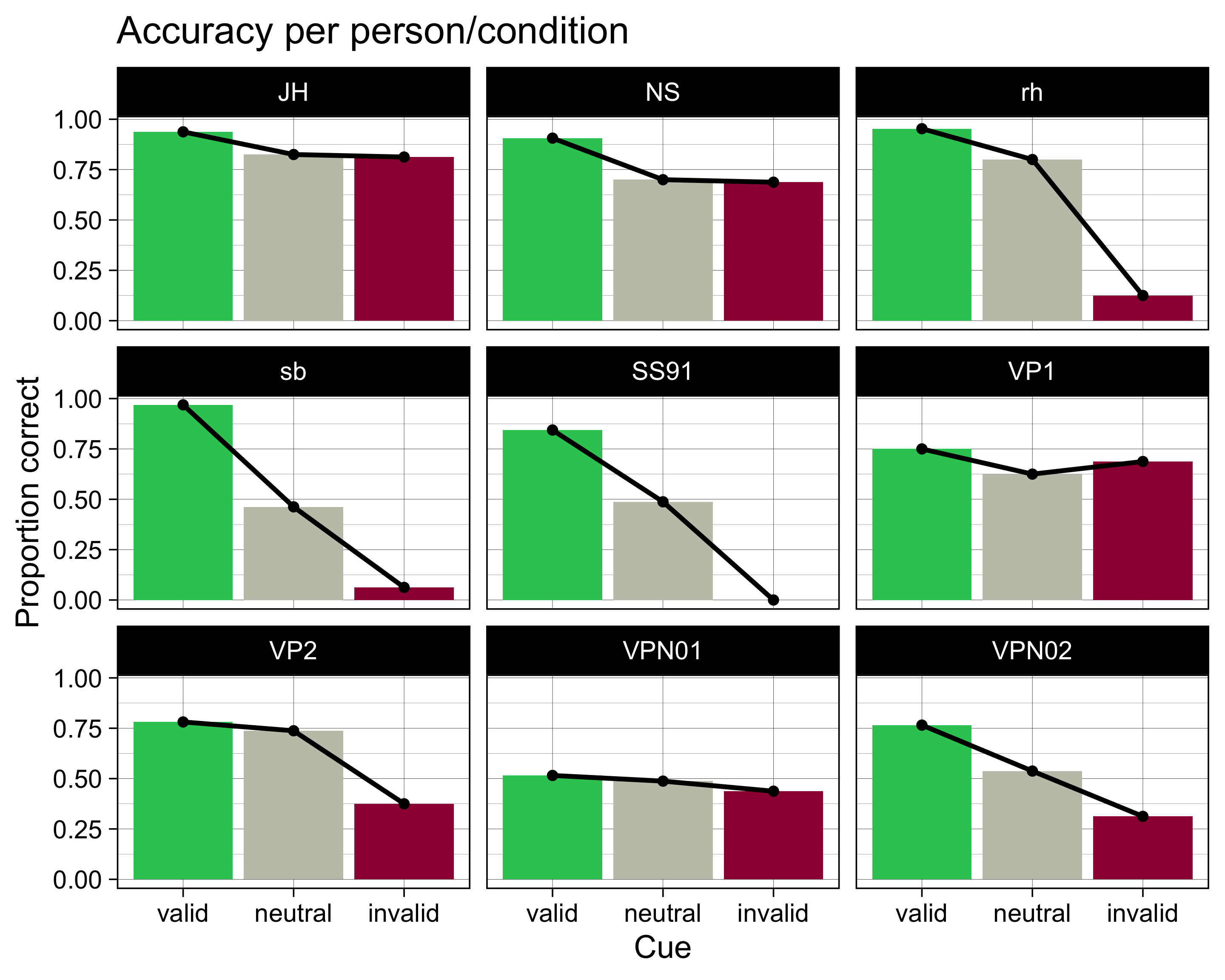

Reuse

https://creativecommons.org/licenses/by/4.0/

Citation

BibTeX citation:

@online{ellis2023,
  author = {Andrew Ellis},
  title = {Daten Importieren: {Teil} 2},
  date = {2023-03-20},
  url = {https://kogpsy.github.io/neuroscicomplabFS23//importing_data-2.html},
  langid = {en}
}

For attribution, please cite this work as:

Andrew Ellis. 2023. “Daten Importieren: Teil 2.” March 20, 2023. https://kogpsy.github.io/neuroscicomplabFS23//importing_data-2.html.

Mehrere Datensätze bearbeiten

Alle Files in einem Ordner auflisten

Mit for-Loop

Mit map und list_rbind

Variablen auswählen und umbennen

Neue Variablen definieren

Korrekte Antworten

Cue-Bedingungsvariable

Daten als CSV speichern

Gruppierungsvariablen

Daten überprüfen

Accuracy pro Person/Bedingung

Visualisieren

Reuse

Citation

Mit `for`-Loop

Mit `map` und `list_rbind`