
library(tidyverse)

d <- read.csv("data/DatasaurusDozen.csv") |>
    filter(condition %in% c("away", "bullseye", "circle", "dino", "dots, star")) |>
    mutate(id = as.factor(id))

d_summary <- d |> group_by(condition) |>
    summarise(mean_x = mean(x),
mean_y = mean(y))4 Data visualization
4.1 Creating graphs with ggplot()
ggstands for grammar of graphics, a framework which aims to describe all components of a graph. The ggplot2-package relies on this framework hence the name. This package is already included in the tidyverse therefore you do not have to install it again. If you load the tidyverse-library, the ggplot2-library is loaded automatically.
A graph contains always:
data
geoms, visible forms (aesthetics) such as points, lines or boxes.
a coordinate systems / mapping describes how data and geoms are linked, also colors or grouping variables are specified here
Further components could be:
statistical parameters
positions
coordinate functions
facets
scales
themes
(we will only cover the contents in italics)
Good to know
For plotting with
ggplot()it is easiest when your data is in long format.What variables do you want to plot (categorical? continuous? …) affects which
geomscan be used. You can try out what is suited with theesquisse-package below or find ideas here.
4.2 Data, geoms and mapping
We start with entering the current data frame and add geoms and mappings (specified with aes()) with arguments such as
ggplot(d_summary, # data
       aes(x = mean_x, y = mean_y)) + # mapping
geom_point() # geom 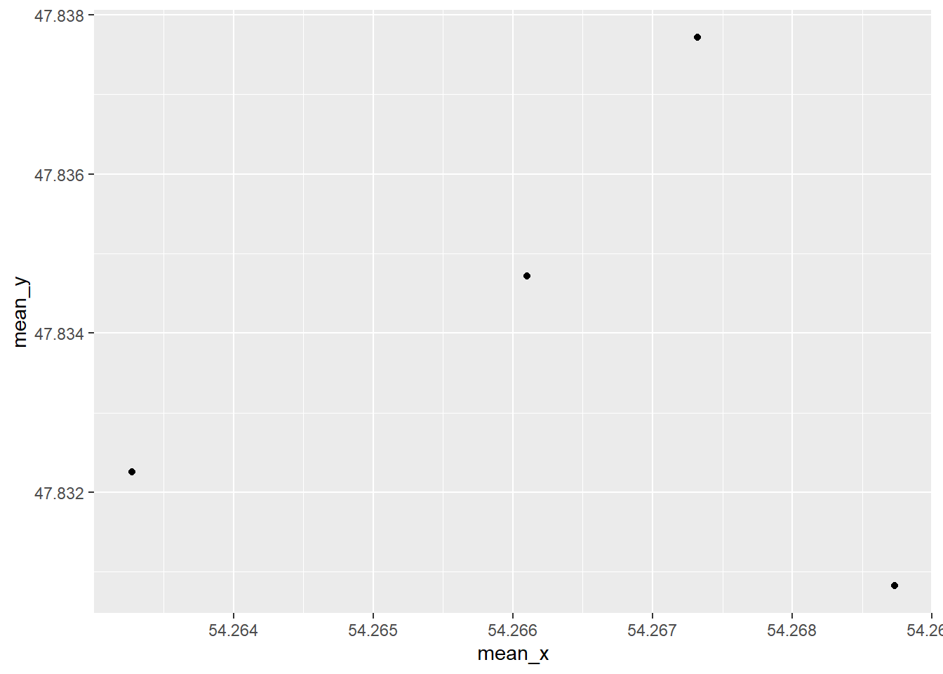
Depending on your variables and what you want to show with your data different geoms are well suited.
Examples of available geoms:
- data points, scatterplots:
geom_point() - lines, tendencies:
geom_line() - histograms:
geom_histogram() - means and standard deviations:
geom_pointrange() - densities:
geom_density() - boxplots:
geom_boxplot() - violin plots:
geom_violin()
4.3 Facets
With facets you can show subsets of your data in different panels
ggplot(d, # data
       aes(x = x, y = y)) + # mapping
    geom_point() + # geom
    facet_grid(~ condition) # facet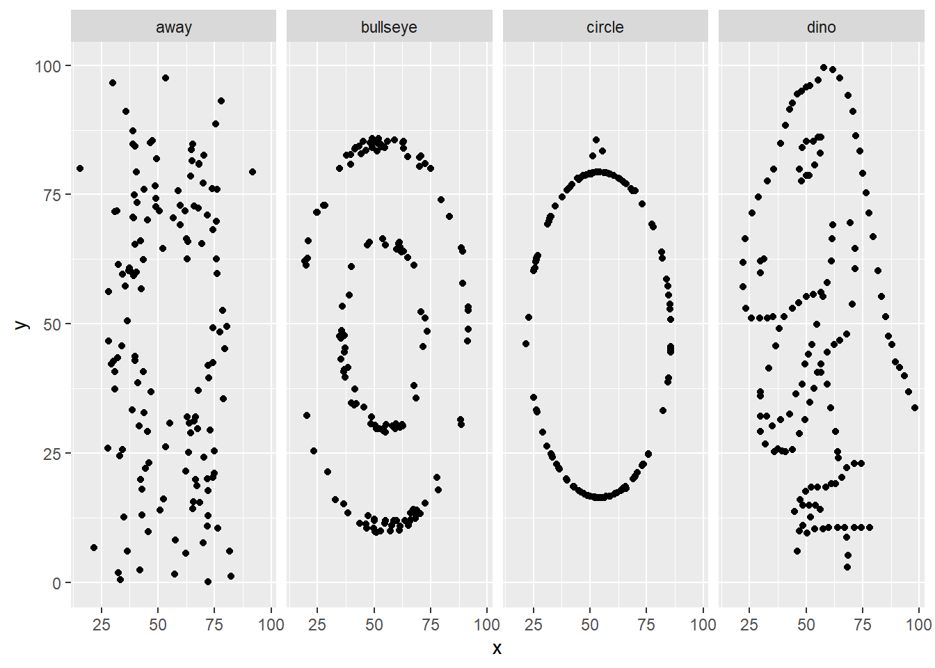
4.4 Themes and labels
ggplot(data = d,
       mapping = aes(x = x,
                     y = y)) +
    geom_point() +
    ggtitle ("Title") +
    labs(title = "Title",
        x = "Variable A  [a.u.]",
        y = "Variable B [a.u.]") +
    theme_minimal() # also theme_classic and theme_minimal are nice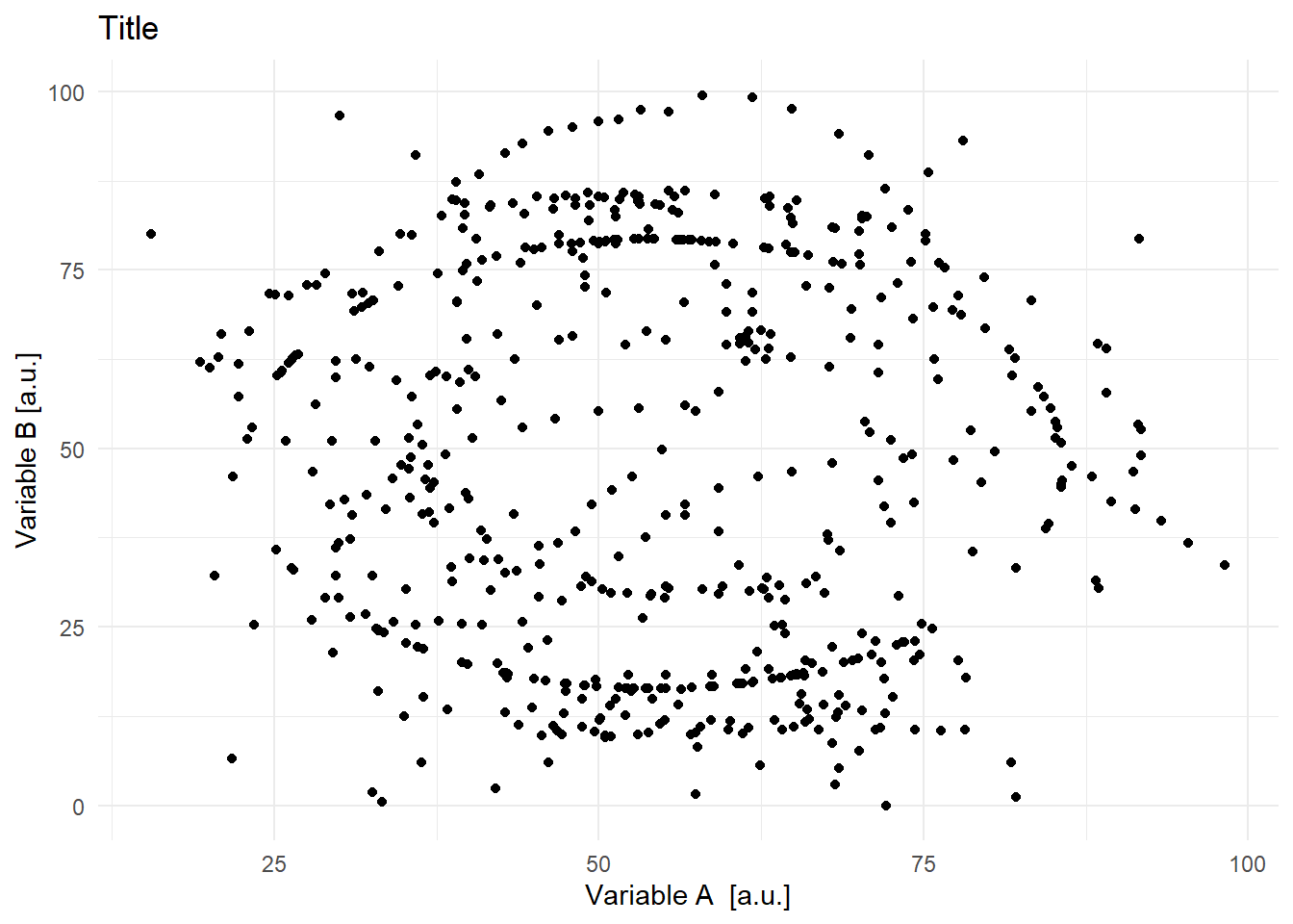
esquisse-package
With this package you can use the data frames in your current environment or load a new one to try out which geoms might be useful
install.packages("esquisse")

esquisse::esquisser() Further helpful ressources:
Start of the PsyTeachR videos by Lisa DeBruine, e.g. Basic Plots, Common Plots and Plot Themes and Customization
Einführung in R by Andrew Ellis and Boris Mayer
Here you find ideas for plots.